注意力机制

注意力提示

固定随机种子

def set_seed(seed: int = 42):
    # Python 内置随机
    random.seed(seed)

    # NumPy 随机
    np.random.seed(seed)

    # PyTorch CPU 随机
    torch.manual_seed(seed)

    # PyTorch GPU 随机(单卡 / 多卡都需要)
    torch.cuda.manual_seed(seed)
    torch.cuda.manual_seed_all(seed)

set_seed(42)

查询、键和值

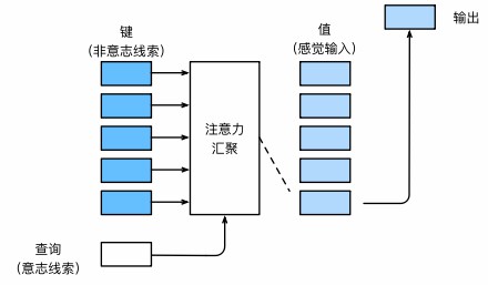
“是否包含自主性提示”将注意力机制与全连接层或汇聚层区别开来

在注意力机制的背景下，自主性提示被称为查询(query)

而非自主性提示作为**键(key)与感官输入(sensory inputs)的值(value)**构成一组 pair 作为输入

给定任何查询，注意力机制通过注意力汇聚(attention pooling) 将非自主性提示的 key 引导至感官输入

在注意力机制中，这些感官输入被称为值(value)

每个值都与一个**键(key)**配对，这可以想象为感官输入的非自主提示

可以通过设计注意力汇聚的方式，便于给定的查询(自主性提示)与键(非自主性提示)进行匹配，这将引导得出最匹配的值(感官输入)

注意力的可视化

平均汇聚层可以被视为输入的加权平均值，其中各输入的权重是一样的

注意力汇聚得到的是加权平均的总和值，其中权重是在给定的查询和不同的键之间计算得出的

import torch
from d2l import torch as d2l

为了可视化注意力权重，需要定义一个show_heatmaps函数

其输入matrices的形状是(num_rows, num_cols, H, W)，每个元素是一个二维矩阵

cmap颜色映射，Reds常用于：

• 权重
• 概率
• 能量 / 强度

#@save
def show_heatmaps(matrices, xlabel, ylabel, titles=None, figsize=(2.5, 2.5),
                  cmap='Reds'):
    """显示矩阵热图"""
    d2l.use_svg_display()
    num_rows, num_cols = matrices.shape[0], matrices.shape[1]
    fig, axes = d2l.plt.subplots(num_rows, num_cols, figsize=figsize,
                                 sharex=True, sharey=True, squeeze=False)
    for i, (row_axes, row_matrices) in enumerate(zip(axes, matrices)):
        for j, (ax, matrix) in enumerate(zip(row_axes, row_matrices)):
            pcm = ax.imshow(matrix.detach().numpy(), cmap=cmap)
            if i == num_rows - 1:
                ax.set_xlabel(xlabel)
            if j == 0:
                ax.set_ylabel(ylabel)
            if titles:
                ax.set_title(titles[j])
    fig.colorbar(pcm, ax=axes, shrink=0.6);

attention_weights = torch.eye(10).reshape((1, 1, 10, 10))
show_heatmaps(attention_weights, xlabel='Keys', ylabel='Queries')

随机生成一个 10×10 矩阵，对每一行做 softmax，得到合法的注意力概率分布

from torch.nn import functional as F
# 随机生成一个 10×10 的原始注意力得分矩阵(logits)
raw_scores = torch.randn(10, 10)  # 得分可为负

# 对每一行做 softmax，确保每一行是合法的概率分布
# 对每一个 Query，所有 Key 的注意力权重加起来等于 1
attention_weights = F.softmax(raw_scores, dim=1)
# 扩展维度以适配 show_heatmaps 的接口
# (1, 1, 10, 10)：表示 1 行 × 1 列 的热图布局
attention_weights_vis = attention_weights.unsqueeze(0).unsqueeze(0)
show_heatmaps(
    attention_weights_vis,
    xlabel='Key Index',
    ylabel='Query Index',
    titles=['Attention Weights'],
    figsize=(4, 4)
)

注意力汇聚:Nadaraya-Watson核回归

了解思想即可，在这里d_model默认为1，所以没有出现Q和K不同维度的问题

查询(自主提示)和键(非自主提示)之间的交互形成了注意力汇聚

注意力汇聚有选择地聚合了值(感官输入)以生成最终的输出

生成数据集

给定的成对的“输入－输出”数据集${(x_1, y_1), \ldots, (x_n, y_n)}$，如何学习$f$来预测任意新输入的输出$\hat{y} = f(x)$

根据下面的非线性函数生成一个人工数据集，其中加入的噪声项为$\epsilon$：
$$
y_i = 2\sin(x_i) + x_i^{0.8} + \epsilon,
$$

n_train = 50  # 训练样本数
x_train, _ = torch.sort(torch.rand(n_train) * 5)   # 排序后的训练样本

def f(x):
    return 2 * torch.sin(x) + x**0.8

y_train = f(x_train) + torch.normal(0.0, 0.5, (n_train,))  # 训练样本的输出
x_test = torch.arange(0, 5, 0.1)  # 测试样本
y_truth = f(x_test)  # 测试样本的真实输出
print(len(x_test))

下面的函数将绘制所有的训练样本(样本由圆圈表示)，不带噪声项的真实数据生成函数(标记为“Truth”)，以及学习得到的预测函数(标记为“Pred”)

def plot_kernel_reg(y_hat):
    d2l.plot(x_test, [y_truth, y_hat], 'x', 'y', legend=['Truth', 'Pred'],
             xlim=[0, 5], ylim=[-1, 5])
    d2l.plt.plot(x_train, y_train, 'o', alpha=0.5)

关于d2l.plot函数：

def has_one_axis(X):  # True if X (tensor or list) has 1 axis
    return (hasattr(X, "ndim") and X.ndim == 1 or isinstance(X, list)
            and not hasattr(X[0], "__len__"))

torch.Tensor和numpy.ndarray有ndim这个属性，Python list 没有

想要list的值扩大不用*，例如[x * 3 for x in X]，用*实现的是复制效果

平均汇聚

基于平均汇聚来计算所有训练样本输出值的平均值
$$
f(x) = \frac{1}{n}\sum_{i=1}^n y_i,
$$

y_hat = torch.repeat_interleave(y_train.mean(), n_test)
plot_kernel_reg(y_hat)

非参数注意力汇聚

根据输入的位置对输出进行加权
$$
f(x) = \sum_{i=1}^n \frac{K(x - x_i)}{\sum_{j=1}^n K(x - x_j)} y_i,
$$
其中是$K$是核(kernel)，公式所描述的估计器被称为Nadaraya-Watson核回归

重写得到一个更加通用的**注意力汇聚(attention pooling)**公式
$$
f(x) = \sum_{i=1}^n \alpha(x, x_i) y_i,
$$
其中$x$是查询，$(x_i, y_i)$是键值对，查询和键之间的关系建模为注意力权重$\alpha(x, x_i)$，这个权重将被分配给每一个对应值$y_i$

对于任何查询，模型在所有键值对注意力权重都是一个有效的概率分布：它们是非负的，并且总和为1

如果把核考虑为高斯核
$$
K(u) = \frac{1}{\sqrt{2\pi}} \exp(-\frac{u^2}{2}).
$$
代入后就能获得：
$$
\begin{split}\begin{aligned} f(x) &=\sum_{i=1}^n \alpha(x, x_i) y_i
\\ &= \sum_{i=1}^n \frac{\exp\left(-\frac{1}{2}(x - x_i)^2\right)}{\sum_{j=1}^n \exp\left(-\frac{1}{2}(x - x_j)^2\right)} y_i
\\&= \sum_{i=1}^n \mathrm{softmax}\left(-\frac{1}{2}(x - x_i)^2\right) y_i. \end{aligned}\end{split}
$$
如果一个键越是接近给定的查询, 那么分配给这个键对应值$y_i$的注意力权重就会越大， 也就“获得了更多的注意力”

Nadaraya-Watson核回归是一个非参数模型，将基于这个非参数的注意力汇聚模型来绘制预测结果

从绘制的结果会发现新的模型预测线是平滑的，并且比平均汇聚的预测更接近真实

# X_repeat的形状:(n_test,n_train),
# 每一行是一个查询(Query)，复制来和所有 Key 对齐
X_repeat = x_test.repeat_interleave(n_train).reshape((-1, n_train))
# x_train包含着键，attention_weights的形状：(n_test,n_train),
# 每一行都包含着要在给定的每个查询的值(y_train)之间分配的注意力权重
attention_weights = F.softmax(-(X_repeat-x_train)**2/2, dim=1)
# y_hat的每个元素都是值的加权平均值，其中的权重是注意力权重
y_hat = torch.matmul(attention_weights, y_train)
plot_kernel_reg(y_hat)

这里测试数据的输入相当于查询，而训练数据的输入相当于键

因此由观察可知“查询-键”对越接近，注意力汇聚的注意力权重就越高

d2l.show_heatmaps(attention_weights.unsqueeze(0).unsqueeze(0),
                  xlabel='Sorted training inputs',
                  ylabel='Sorted testing inputs')

带参数注意力汇聚

非参数的Nadaraya-Watson核回归具有一致性的优点：如果有足够的数据，此模型会收敛到最优结果

在下面的查询和键之间的距离乘以可学习参数$w$
$$
\begin{split}\begin{aligned}f(x) &= \sum_{i=1}^n \alpha(x, x_i) y_i \\
&= \sum_{i=1}^n \frac{\exp\left(-\frac{1}{2}((x - x_i)w)^2\right)}{\sum_{j=1}^n \exp\left(-\frac{1}{2}((x - x_j)w)^2\right)} y_i \\
&= \sum_{i=1}^n \mathrm{softmax}\left(-\frac{1}{2}((x - x_i)w)^2\right) y_i.\end{aligned}\end{split}
$$

批量矩阵乘法

为了更有效地计算小批量数据的注意力，可以利用深度学习开发框架中提供的批量矩阵乘法

假设第一个小批量数据包含$n$个矩阵$\mathbf{X}_1,\ldots, \mathbf{X}_n$，形状为$a\times b$，第二个小批量包含$n$个矩阵，$\mathbf{Y}_1, \ldots, \mathbf{Y}_n$，形状为$b\times c$，

它们的批量矩阵乘法得到$n$个矩阵$\mathbf{X}_1\mathbf{Y}_1, \ldots, \mathbf{X}_n\mathbf{Y}_n$，形状为$a\times c$

假定两个张量的形状分别是$(n,a,b)$和$(n,b,c)$，它们的批量矩阵乘法输出的形状为$(n,a,c)$

为什么要引入“批量矩阵乘法”？

深度学习里几乎所有东西都是“成批”的，例如在 Attention 中：

• attention_weights：(batch, query_len, key_len)
• values：(batch, key_len, d)

输出是：

(batch, query_len, d)

本质上就是批量矩阵乘法

在注意力机制的背景中，可以使用小批量矩阵乘法来计算小批量数据中的加权平均值

weights = torch.ones((2, 10)) * 0.1 # 2个batch，均匀注意力
values = torch.arange(20.0).reshape((2, 10)) # 2个batch，每个batch有10个value
torch.bmm(weights.unsqueeze(1), values.unsqueeze(-1))
# weights.unsqueeze(1)把(2, 10)变为(batch×1×key_len)，1对应query数量
# values.unsqueeze(-1)把(2, 10)变为(batch×key_len×1)，1对应value_dim
# 输出结果为(2,1,1)

tensor([[[ 4.5000]],

        [[14.5000]]])

定义模型

repeat_interleave 只能把数据“拉平成一维重复”，真正需要的是一个二维的
(查询个数, 键的个数) 矩阵

使用小批量矩阵乘法，定义Nadaraya-Watson核回归的带参数版本为

from torch import nn
class NWKernelRegression(nn.Module):
    def __init__(self, **kwargs):
        super().__init__(**kwargs)
        self.w = nn.Parameter(torch.rand((1,), requires_grad=True)) # 这里w是一个标量，到transformer成为二维

    def forward(self, queries, keys, values):
        # queries和attention_weights的形状为(查询个数，“键－值”对个数)
        queries = queries.repeat_interleave(keys.shape[1]).reshape((-1, keys.shape[1]))
        self.attention_weights = F.softmax(
            -((queries - keys) * self.w)**2 / 2, dim=1)
        # values的形状为(查询个数，“键－值”对个数)
        return torch.bmm(self.attention_weights.unsqueeze(1),
                         values.unsqueeze(-1)).reshape(-1) # 去掉“人为保留的 1×1 维度”，把结果还原成一维向量

训练

将训练数据集变换为键和值用于训练注意力模型

在带参数的注意力汇聚模型中，任何一个训练样本的输入都会和除自己以外的所有训练样本的“键－值”对进行计算，从而得到其对应的预测输出

# X_tile的形状:(n_train，n_train)，每一行都包含着相同的训练输入
X_tile = x_train.repeat((n_train, 1))
# Y_tile的形状:(n_train，n_train)，每一行都包含着相同的训练输出
Y_tile = y_train.repeat((n_train, 1))
# keys的形状:('n_train'，'n_train'-1)，每个 query 对应 n_train-1 个 key
# 构造“掩码”，去掉对角线
keys = X_tile[(1 - torch.eye(n_train)).type(torch.bool)].reshape((n_train, -1))
# values的形状:('n_train'，'n_train'-1)，每个 query 对应 n_train-1 个 value
values = Y_tile[(1 - torch.eye(n_train)).type(torch.bool)].reshape((n_train, -1))
# 第 i 行 = 用来预测第 i 个样本的“所有其他输入”

训练带参数的注意力汇聚模型时，使用平方损失函数和随机梯度下降

反向传播算法Adam和SGD有什么区别?

SGD：只看“当前梯度”，走得朴素但稳定

Adam：记住“历史梯度的方向和大小”，走得快但更激进

维度	SGD	Adam
是否记历史	否	是
学习率	全局一个	参数自适应
对尺度敏感	很敏感	不敏感
收敛速度	慢	快
稳定性	高	初期可能不稳
泛化(经验)	常更好	有时略差
超参数	少	多

net = NWKernelRegression()
loss = nn.MSELoss(reduction='none')
trainer = torch.optim.SGD(net.parameters(), lr=0.5)
animator = d2l.Animator(xlabel='epoch', ylabel='loss', xlim=[1, 5])

for epoch in range(5):
    trainer.zero_grad()
    l = loss(net(x_train, keys, values), y_train)
    l.sum().backward()
    trainer.step()
    print(f'epoch {epoch + 1}, loss {float(l.sum()):.6f}')
    animator.add(epoch + 1, float(l.sum()))

举个例子：

x_train = [1 2 3 4]  # 也就是q
keys = 
	[
		[2 3 4]
		[1 3 4]
		[1 2 4]
		[1 2 3]
	]
queries = 
	[
		[1 1 1]
		[2 2 2]
		[3 3 3]
		[4 4 4]
	]
# 这样才能让queries - keys获得距离
# 行数始终为n_train，但列数会因为避免和自己计算而减1

训练完带参数的注意力汇聚模型后可以发现：在尝试拟合带噪声的训练数据时，预测结果绘制的线不如之前非参数模型的平滑

# keys的形状:(n_test，n_train)，每一行包含着相同的训练输入(例如，相同的键)
keys = x_train.repeat((n_test, 1))
# value的形状:(n_test，n_train)
values = y_train.repeat((n_test, 1))
y_hat = net(x_test, keys, values).unsqueeze(1).detach()
plot_kernel_reg(y_hat)

为什么新的模型更不平滑了呢？看一下输出结果的绘制图：与非参数的注意力汇聚模型相比，带参数的模型加入可学习的参数后，曲线在注意力权重较大的区域变得更不平滑

思考题

• 在带参数的注意力汇聚的实验中学习得到的参数的价值是什么？为什么在可视化注意力权重时，它会使加权区域更加尖锐？

  通过学习参数，自动学会了“相似性的尺度与判别标准”

  w 小：核函数宽；注意力分布平；很多点一起平均 → 低方差，高偏差

  w 大：核函数窄；权重集中在少数点 → 低偏差，高方差

  因为可学习参数放大了相似度差异，而 softmax 会对这种差异做指数级放大，两者叠加的结果就是——权重集中到极少数位置，在可视化中表现为加权区域更加尖锐，所以transformer里加入了$\sqrt d$控制 score 的尺度，防止过度尖锐

• 为本节的核回归设计一个新的带参数的注意力汇聚模型。训练这个新模型并可视化其注意力权重

  class ParametricKernelAttention(nn.Module):
      def __init__(self):
          super().__init__()
          # log_sigma 保证 sigma > 0(数值稳定)
          self.log_sigma = nn.Parameter(torch.zeros(1))
          # 可学习偏置
          self.bias = nn.Parameter(torch.zeros(1))
  
      def forward(self, queries, keys, values):
          """
          queries: (n_query,)
          keys:    (n_query, n_kv)
          values:  (n_query, n_kv)
          """
          n_kv = keys.shape[1]
  
          # (n_query, n_kv)
          queries = queries.repeat_interleave(n_kv).reshape(-1, n_kv)
  
          sigma = torch.exp(self.log_sigma)
  
          # 注意力打分
          scores = -(queries - keys) ** 2 / (2 * sigma ** 2) + self.bias
  
          # 注意力权重
          self.attention_weights = F.softmax(scores, dim=1)
  
          # 加权求和
          out = torch.bmm(
              self.attention_weights.unsqueeze(1),
              values.unsqueeze(-1)
          ).reshape(-1)
  
          return out
      
  
  net = ParametricKernelAttention()
  loss = nn.MSELoss(reduction='none')
  trainer = torch.optim.Adam(net.parameters(), lr=0.1)
  
  num_epochs = 20
  losses = []
  
  for epoch in range(num_epochs):
      trainer.zero_grad()
      y_hat = net(x_train, keys, values)
      l = loss(y_hat, y_train)
      l.sum().backward()
      trainer.step()
  
      losses.append(float(l.sum()))
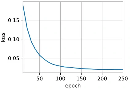
      print(f'epoch {epoch+1}, loss {float(l.sum()):.6f}')

  训练出来的更稳一些，优化空间更“正交”，梯度更稳定，也更容易找到好解

  

注意力评分函数

Nadaraya-Watson使用高斯核来对查询和键之间的关系建模，高斯核指数部分可以视为注意力评分函数，简称评分函数

然后把这个函数的输出结果输入到softmax函数中进行运算，注意力汇聚的输出就是基于这些注意力权重的值的加权和

由于注意力权重是概率分布，因此加权和其本质上是加权平均值

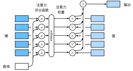
假设有一个查询$\mathbf{q} \in \mathbb{R}^q$和$m$个“键－值”对$(\mathbf{k}_1, \mathbf{v}_1), \ldots, (\mathbf{k}_m, \mathbf{v}_m)$，其中$\mathbf{k}_i \in \mathbb{R}^k$，$\mathbf{v}_i \in \mathbb{R}^v$

注意力汇聚函数就被表示成值的加权和
$$
f(\mathbf{q}, (\mathbf k_1, \mathbf v_1 ), \ldots, (\mathbf k_m, \mathbf v_m)) = \sum_{i=1}^m \alpha(\mathbf q, \mathbf k_i) \mathbf v_i \in \mathbb{R}^v
$$
其中查询和键的注意力权重(标量)是通过注意力评分函数将两个向量映射成标量，再经过softmax运算得到的
$$
\alpha(\mathbf{q}, \mathbf k_i) = \mathrm{softmax}(a(\mathbf{q}, \mathbf k_i)) = \frac{\exp(a(\mathbf{q}, \mathbf k_i))}{\sum_{j=1}^m \exp(a(\mathbf{q}, \mathbf k_j))} \in \mathbb{R}.
$$

掩蔽softmax操作

softmax操作用于输出一个概率分布作为注意力权重，在某些情况下，并非所有的值都应该被纳入到注意力汇聚中

比如某些文本序列被填充了没有意义的特殊词元，为了仅将有意义的词元作为值来获取注意力汇聚，可以指定一个有效序列长度，以便在计算softmax时过滤掉超出指定范围的位置

#@save
def masked_softmax(X, valid_lens):
    """通过在最后一个轴上掩蔽元素来执行softmax操作"""
    # X:3D张量，valid_lens:1D或2D张量
    # X.shape == (batch_size, num_queries, num_keys)
    if valid_lens is None:
        return nn.functional.softmax(X, dim=-1)
    else:
        shape = X.shape
        if valid_lens.dim() == 1: # 每个 batch 一个 有效 key 长度
            valid_lens = torch.repeat_interleave(valid_lens, shape[1]) # 实现拉成(B×Q,)
        else: # 每个 batch 的每个 query 有自己的有效 key 长度
            valid_lens = valid_lens.reshape(-1) # 拉成(B×Q,)，匹配后面的X.reshape(-1, shape[-1])
        
        # 最后一轴上被掩蔽的元素使用一个非常大的负值替换，从而其softmax输出为0
        # 因为sequence_mask输入(N, L)，所以要把batch和Q合并，K不变
        X = d2l.sequence_mask(X.reshape(-1, shape[-1]), valid_lens,
                              value=-1e6)
        # 从(B×Q, K) → (B, Q, K)
        return nn.functional.softmax(X.reshape(shape), dim=-1)

考虑由两个矩阵表示的样本，这两个样本的有效长度分别为2和3，经过掩蔽softmax操作，超出有效长度的值都被掩蔽为0

masked_softmax(torch.rand(2, 2, 4), torch.tensor([2, 3]))

tensor([[[0.5396, 0.4604, 0.0000, 0.0000],
         [0.5120, 0.4880, 0.0000, 0.0000]],

        [[0.3211, 0.3711, 0.3078, 0.0000],
         [0.2700, 0.2769, 0.4531, 0.0000]]])

同样，也可以使用二维张量，为矩阵样本中的每一行指定有效长度

masked_softmax(torch.rand(2, 2, 4), torch.tensor([[1, 3], [2, 4]]))

tensor([[[1.0000, 0.0000, 0.0000, 0.0000],
         [0.3466, 0.3790, 0.2744, 0.0000]],

        [[0.3545, 0.6455, 0.0000, 0.0000],
         [0.1659, 0.3488, 0.1922, 0.2931]]])

加性注意力

当查询Q和键K是不同维度的矢量时，可以使用加性注意力作为评分函数

Q和K维度相同 指的是 $d_q = d_k$

Q.shape = (batch_size, num_queries, d_q)
K.shape = (batch_size, num_keys,    d_k)
V.shape = (batch_size, num_keys,    d_v)

值的特征维度和键/查询的特征维度可以不一样，但值的序列长度必须和键的相同

给定查询$\mathbf{q} \in \mathbb{R}^q$和键$\mathbf{k} \in \mathbb{R}^k$，加性注意力的评分函数为
$$
a(\mathbf q, \mathbf k) = \mathbf w_v^\top \text{tanh}(\mathbf W_q\mathbf q + \mathbf W_k \mathbf k) \in \mathbb{R},
$$
将查询和键连结起来后输入到一个多层感知机(MLP)中，感知机包含一个隐藏层，通过使用$\tanh$作为激活函数，并且禁用偏置项

禁用偏置项的情况：

• 紧跟 BatchNorm / LayerNorm 的线性层或卷积层，前一层的 bias 会被完全抵消，属于冗余参数

  Conv + BN：Conv 通常 bias=False

  Linear + LN：Linear 通常 bias=False

• 注意力机制中的打分网络

  打分函数关注的是 相对相似度，加 bias 会引入与$q,k$无关的常数偏好

• 点积注意力中的线性映射

  在 Transformer 中，W_q, W_k, W_v 通常不带 bias，因为后面跟 LayerNorm

一般在最终分类 / 回归输出层以及中间的 MLP 表示学习层(无 BN/LN)时加入bias

#@save
class AdditiveAttention(nn.Module):
    """加性注意力"""
    def __init__(self, key_size, query_size, num_hiddens, dropout, **kwargs):
        super().__init__(**kwargs)
        # 把Q和K映射到相同维度，这是“加性注意力”能处理不同维度 Q/K 的关键
        self.W_q = nn.Linear(query_size, num_hiddens, bias=False)
        self.W_k = nn.Linear(key_size, num_hiddens, bias=False)
        # 把“特征向量”压成“相似度分数”
        self.W_v = nn.Linear(num_hiddens, 1, bias=False)
        self.dropout = nn.Dropout(dropout)

    def forward(self, queries, keys, values, valid_lens):
        queries, keys = self.W_q(queries), self.W_k(keys)
        # queries.shape = (batch_size, num_queries, num_hiddens)
        # keys.shape    = (batch_size, num_kv, num_hiddens)
        # 在维度扩展后，
        # queries.shape = (batch_size, num_queries, 1, num_hiddens)
        # keys.shape    = (batch_size, 1, num_kv, num_hiddens)
        # 使用广播方式进行求和
        features = queries.unsqueeze(2) + keys.unsqueeze(1)
        # features.shape = (batch_size, num_queries, num_kv, num_hiddens)
        features = torch.tanh(features)
        # self.w_v仅有一个输出，因此从形状中移除最后那个维度
        # scores的形状：(batch_size， num_queries, num_kv)
        scores = self.W_v(features).squeeze(-1)
        self.attention_weights = masked_softmax(scores, valid_lens)
        # values的形状：(batch_size, num_kv, value_size)
        return torch.bmm(self.dropout(self.attention_weights), values)

输出张量为(batch_size, num_queries, value_size)

点积注意力要求查询和键在特征维度上完全一致，否则内积无法定义

而加性注意力通过对查询Q和键K分别做线性映射，把它们投影到同一隐藏空间，从而在原始维度不同的情况下仍然可以计算相似度

查询、键和值的形状为**[批量大小，步数或词元序列长度，特征大小]→(batch_size, num_len, d_k)**

注意力汇聚输出的形状为**[批量大小，查询的步数，值的维度]→(batch_size, num_queries, value_size)**

对比Transformer

维度	AdditiveAttention	Transformer Attention
相似度	MLP + tanh (加性)	点积(极致并行和效率)
Q/K 原始维度	可不同	必须相同
是否用 MLP	✅	❌
是否需要 √d 缩放	❌	✅
多头	❌	✅
表达灵活性	高	中
计算效率	低	极高
并行能力	一般	极强
适合时代	RNN 时代	大模型时代

用一个小例子来演示上面的AdditiveAttention类

queries, keys = torch.normal(0, 1, (2, 1, 20)), torch.ones((2, 10, 2))
# values的小批量，两个值矩阵是相同的
values = torch.arange(40, dtype=torch.float32).reshape(1, 10, 4).repeat(
    2, 1, 1)
valid_lens = torch.tensor([2, 6])

attention = AdditiveAttention(key_size=2, query_size=20, num_hiddens=8,
                              dropout=0.1)
attention.eval()
attention(queries, keys, values, valid_lens)

tensor([[[ 2.0000,  3.0000,  4.0000,  5.0000]],

        [[10.0000, 11.0000, 12.0000, 13.0000]]], grad_fn=<BmmBackward0>)

加性注意力并没有“选择”任何 key，因为所有 key 是等价的，只剩下 mask 在起作用，注意力机制退化成了对前 valid_lens[i] 个 value 做平均

values =
[[[ 0,  1,  2,  3],
  [ 4,  5,  6,  7],
  [ 8,  9, 10, 11],
  [12, 13, 14, 15],
  [16, 17, 18, 19],
  [20, 21, 22, 23],
  [24, 25, 26, 27],
  [28, 29, 30, 31],
  [32, 33, 34, 35],
  [36, 37, 38, 39]]]

第 0 个 batchvalid_lens[0] = 2

[0.5, 0.5, 0, 0, 0, 0, 0, 0, 0, 0]

前 2 个 value 的平均

[(0+4)/2, (1+5)/2, (2+6)/2, (3+7)/2]
= [2, 3, 4, 5]

第 1 个 batchvalid_lens[0] = 6

[1/6, 1/6, 1/6, 1/6, 1/6, 1/6, 0, 0, 0, 0]

[(0+4+8+12+16+20)/6,
 (1+5+9+13+17+21)/6,
 (2+6+10+14+18+22)/6,
 (3+7+11+15+19+23)/6]
= [10, 11, 12, 13]

尽管加性注意力包含了可学习的参数，但由于本例子中每个键都是相同的，所以注意力权重是均匀的，由指定的有效长度决定

缩放点积注意力

使用点积可以得到计算效率更高的评分函数，但是点积操作要求查询和键具有相同的特征维度

为了方便表述，$d_q=d_k$后面统一用$d_k$

将点积除以$\sqrt{d}$，则**缩放点积注意力(scaled dot-product attention)**评分函数为
$$
a(\mathbf q, \mathbf k) = \mathbf{q}^\top \mathbf{k} /\sqrt{d}.
$$
这里和 Transformer 完全一致，是点积注意力在高维下必须引入的数值稳定性修正，没有这一项点积注意力在高维下会数值失控

从统计角度看
$$
\mathbf{q}^{\top} \mathbf{k}=\sum_{i=1}^{d} q_i k_i
$$
维度越大，点积的波动越大，会直接把 softmax 推进饱和区，softmax 变成近似 one-hot，梯度几乎为 0，训练会变得极其不稳定，除以$\sqrt{d}$ 本质上是在做方差归一化

换到小批量写法，基于$n$查询和$m$个键-值对计算注意力，其中查询和键的特征维度为$d_k$，值的特征维度为$d_v$

查询$\mathbf Q\in\mathbb R^{n\times d}$，键$\mathbf K\in\mathbb R^{m\times d}$，值$\mathbf V\in\mathbb R^{m\times v}$ 缩放点积注意力是
$$
\mathrm{softmax}\left(\frac{\mathbf Q \mathbf K^\top }{\sqrt{d}}\right) \mathbf V \in \mathbb{R}^{n\times v}.
$$
缩放点积注意力的实现使用了暂退法进行模型正则化

import math
#@save
class DotProductAttention(nn.Module):
    """缩放点积注意力"""
    def __init__(self, dropout, **kwargs):
        super().__init__(**kwargs)
        self.dropout = nn.Dropout(dropout)
    # queries：(batch_size，num_queries，d_k)
    # keys：   (batch_size，num_kv，d_k)
    # values： (batch_size，num_kv，d_v)
    # valid_lens :(batch_size，) or (batch_size，num_queries)
    def forward(self, queries, keys, values, valid_lens=None):
        d = queries.shape[-1]
        # 设置transpose_b=True为了交换keys的最后两个维度
        # 因为之前写的时候都会专门加维度点积，现在是不加直接交换维度点积
        scores = torch.bmm(queries, keys.transpose(1,2)) / math.sqrt(d)
        self.attention_weights = masked_softmax(scores, valid_lens)
        # attention_weights: (batch_size, num_queries, num_kv)
        return torch.bmm(self.dropout(self.attention_weights), values)
    	# 输出: (batch_size, num_queries, d_v)

演示上述的DotProductAttention类

使用与先前加性注意力例子中相同的键、值和有效长度

queries = torch.normal(0, 1, (2, 1, 2))
keys =  torch.ones((2, 10, 2))
values = torch.arange(40, dtype=torch.float32).reshape(1, 10, 4).repeat(
    2, 1, 1)
valid_lens = torch.tensor([2, 6])
attention = DotProductAttention(dropout=0.5)
attention.eval()
attention(queries, keys, values, valid_lens)

tensor([[[ 2.0000,  3.0000,  4.0000,  5.0000]],

        [[10.0000, 11.0000, 12.0000, 13.0000]]])

输出结果应该是相同的

查询的维度和内容只有在键之间存在差异时才会影响注意力结果；当所有键在注意力空间中等价时，注意力机制退化为均匀加权，此时无论查询维度多大、取值多复杂，输出结果都不会发生变化

情况	Query 是否影响输出
所有 key 完全相同	❌ 不影响
key 不同，但 query=0	❌ 不影响
key 不同，query 有区分	✅ 强烈影响
query 维度↑，key 不变	❌ 仍不影响
query 维度↑，key 有结构	✅ 影响更丰富

如果修改键，不再相同，可加性注意力和缩放的“点－积”注意力不再产生相同的结果

keys = torch.arange(20, dtype=torch.float32)\
            .reshape(1, 10, 2)\
            .repeat(2, 1, 1)

在加性注意力下，score 有差异，但差异不大，权重 ≈ “接近均匀、略有偏向”

attention_weights ≈
[0.476, 0.524, 0, 0, 0, 0, 0, 0, 0, 0]   # batch 0

tensor([[[ 2.0962,  3.0962,  4.0962,  5.0962]],

        [[ 9.6081, 10.6081, 11.6081, 12.6081]]])

在缩放点积注意力下，权重高度集中

attention_weights ≈
[0.85, 0.15, 0, 0, 0, 0, 0, 0, 0, 0]   # batch 0

几乎就是第一个 value，加一点点第二个

tensor([[[0.2894, 1.2894, 2.2894, 3.2894]],

        [[4.4147, 5.4147, 6.4147, 7.4147]]])

项目	加性注意力	点积注意力
打分函数	MLP + tanh	内积
数值压缩	有(tanh)	无
score 差异	小	大
softmax 后	平滑	尖锐
输出表现	接近均值	偏向少数 key
适用场景	适合大规模与精确对齐	适合大规模与精确对齐
图片

所以点积注意力可能会过度关注某些位置，这也就是为什么transformer引入多头

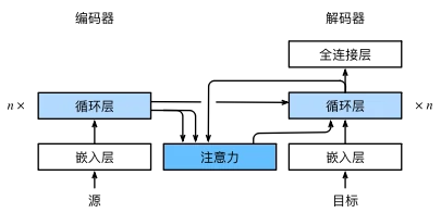
Bahdanau 注意力

Bahdanau等人提出了一个没有严格单向对齐限制的 可微注意力模型，在预测词元时，如果不是所有输入词元都相关，模型将仅对齐(或参与)输入序列中与当前预测相关的部分

模型

定义注意力解码器

AttentionDecoder类定义了带有注意力机制解码器的基本接口

#@save
class AttentionDecoder(d2l.Decoder):
    """带有注意力机制解码器的基本接口"""
    def __init__(self, **kwargs):
        super().__init__(**kwargs)

    @property
    # 所有带注意力的 Decoder，都应该有一个 attention_weights 这个属性
    def attention_weights(self):
        raise NotImplementedError

在接下来的Seq2SeqAttentionDecoder类中实现带有Bahdanau注意力的循环神经网络解码器

首先，初始化解码器的状态，需要下面的输入：

1. 编码器在所有时间步的最终层隐状态，将作为注意力的键和值；
2. 上一时间步的编码器全层隐状态，将作为初始化解码器的隐状态；
3. 编码器有效长度(排除在注意力池中填充词元)

在每个解码时间步骤中，解码器上一个时间步的最终层隐状态将用作查询，注意力输出和输入嵌入都连结为循环神经网络解码器的输入

num_steps：一句话有多长(时间轴)

num_hiddens：模型在每个位置能记住多少信息(空间轴)

class Seq2SeqAttentionDecoder(AttentionDecoder):
    def __init__(self, vocab_size, embed_size, num_hiddens, num_layers,
                 dropout=0, **kwargs):
        super().__init__(**kwargs)
        self.attention = d2l.AdditiveAttention(num_hiddens, dropout)
        # 把 token id → embed_size 向量
        self.embedding = nn.Embedding(vocab_size, embed_size)
        # GRU 输入维度是 embed_size + num_hiddens
        # decoder 每个时间步喂给 GRU 的输入不是单纯的 embedding
        # 当前目标词的 embedding + 当前注意力得到的 context
        self.rnn = nn.GRU(
            embed_size + num_hiddens, num_hiddens, num_layers,
            dropout=dropout)
        # 将 GRU 输出的 hidden → 词表维度 logits(未softmax)
        self.dense = nn.Linear(num_hiddens, vocab_size)

    # state 里保存的 enc_outputs 的维度排列必须与 attention 的实现期望一致
    def init_state(self, enc_outputs, enc_valid_lens, *args):
        # enc_outputs：encoder 每个时间步的输出(给 attention 当 key/value)
        # hidden_state：encoder 的最终隐藏状态(给 decoder 当初始 hidden_state)
        # enc_valid_lens：每个样本真实长度(mask padding，防止注意力看 padding)
        outputs, hidden_state = enc_outputs
        # outputs的形状为(batch_size，num_steps，num_hiddens).
        # decoder 的实现通常是“时间步优先”，所以将outputs的时间步放到最开头
        # hidden_state的形状为(num_layers，batch_size，num_hiddens)
        return (outputs.permute(1, 0, 2), hidden_state, enc_valid_lens)

    def forward(self, X, state):
        # enc_outputs的形状为(batch_size,num_steps,num_hiddens).
        enc_outputs, hidden_state, enc_valid_lens = state
        # 输出X的形状为(num_steps,batch_size,embed_size)
        X = self.embedding(X).permute(1, 0, 2)
        outputs, self._attention_weights = [], []
        for x in X:
            # 在 decoder 里每个时间步只算 一个 query
            # query的形状为(batch_size,1,num_hiddens)
            query = torch.unsqueeze(hidden_state[-1], dim=1)
            # context的形状为(batch_size,1,num_hiddens)
            context = self.attention(
                query, enc_outputs, enc_outputs, enc_valid_lens)
            # 在特征维度上连结
            x = torch.cat((context, torch.unsqueeze(x, dim=1)), dim=-1)
            # 将x变形为(1,batch_size,embed_size+num_hiddens)
            out, hidden_state = self.rnn(x.permute(1, 0, 2), hidden_state)
            outputs.append(out)
            self._attention_weights.append(self.attention.attention_weights)
        # 全连接层变换后，outputs的形状为
        # (num_steps,batch_size,vocab_size)
        outputs = self.dense(torch.cat(outputs, dim=0))
        return outputs.permute(1, 0, 2), [enc_outputs, hidden_state,
                                          enc_valid_lens]

    @property
    def attention_weights(self):
        return self._attention_weights

使用包含7个时间步的4个序列输入的小批量测试Bahdanau注意力解码器

encoder = d2l.Seq2SeqEncoder(vocab_size=10, embed_size=8, num_hiddens=16,
                             num_layers=2)
encoder.eval()
decoder = Seq2SeqAttentionDecoder(vocab_size=10, embed_size=8, num_hiddens=16,
                                  num_layers=2)
decoder.eval()
X = torch.zeros((4, 7), dtype=torch.long)  # (batch_size,num_steps)
state = decoder.init_state(encoder(X), None)
output, state = decoder(X, state)
output.shape, len(state), state[0].shape, len(state[1]), state[1][0].shape

(torch.Size([4, 7, 10]), 3, torch.Size([4, 7, 16]), 2, torch.Size([4, 16]))

训练

指定超参数，实例化一个带有Bahdanau注意力的编码器和解码器，并对这个模型进行机器翻译训练

class EncoderDecoderCompat(nn.Module):
    def __init__(self, encoder, decoder):
        super().__init__()
        self.encoder = encoder
        self.decoder = decoder

    def forward(self, enc_X, dec_X, enc_valid_lens):
        # Encoder
        enc_outputs = self.encoder(enc_X, enc_valid_lens)
        # Decoder init
        dec_state = self.decoder.init_state(enc_outputs, enc_valid_lens)
        # 必须返回 (Y_hat, state)
        return self.decoder(dec_X, dec_state)

# 超参数
embed_size, num_hiddens, num_layers, dropout = 32, 32, 2, 0.1
batch_size, num_steps = 64, 10
lr, num_epochs, device = 0.005, 250, d2l.try_gpu()

# 数据
train_iter, src_vocab, tgt_vocab = d2l.load_data_nmt(batch_size, num_steps)

# Encoder / Decoder
encoder = d2l.Seq2SeqEncoder(
    len(src_vocab), embed_size, num_hiddens, num_layers, dropout
)
decoder = Seq2SeqAttentionDecoder(
    len(tgt_vocab), embed_size, num_hiddens, num_layers, dropout
)

net = EncoderDecoderCompat(encoder, decoder)

# 训练
d2l.train_seq2seq(
    net, train_iter, lr, num_epochs, tgt_vocab, device
)

loss 0.020, 10635.4 tokens/sec on cpu

模型训练后，用它将几个英语句子翻译成法语并计算它们的BLEU分数

engs = ['go .', "i lost .", 'he\'s calm .', 'i\'m home .']
fras = ['va !', 'j\'ai perdu .', 'il est calme .', 'je suis chez moi .']
for eng, fra in zip(engs, fras):
    translation, dec_attention_weight_seq = d2l.predict_seq2seq(
        net, eng, src_vocab, tgt_vocab, num_steps, device, True)
    print(f'{eng} => {translation}, ',
          f'bleu {d2l.bleu(translation, fra, k=2):.3f}')

go . => va !,  bleu 1.000
i lost . => j'ai perdu .,  bleu 1.000
he's calm . => il est paresseux .,  bleu 0.658
i'm home . => je suis chez moi .,  bleu 1.000

训练结束后，下面通过可视化注意力权重会发现，每个查询都会在键值对上分配不同的权重，这说明在每个解码步中，输入序列的不同部分被选择性地聚集在注意力池中

attention_weights = torch.cat([step[0][0][0] for step in dec_attention_weight_seq], 0).reshape((
    1, 1, -1, num_steps))
    # 加上一个包含序列结束词元
d2l.show_heatmaps(
    attention_weights[:, :, :, :len(engs[-1].split()) + 1].cpu(),
    xlabel='Key positions', ylabel='Query positions')

多头注意力

给定相同的查询、键和值的集合时，希望模型可以基于相同的注意力机制学习到不同的行为，然后将不同的行为作为知识组合起来，捕获序列内各种范围的依赖关系

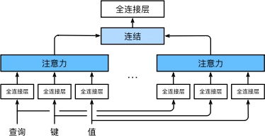
可以用独立学习得到的$h$组不同的线性投影(linear projections)来变换查询、键和值

然后，这$h$组变换后的查询、键和值将并行地送到注意力汇聚中，最后将这$h$个注意力汇聚的输出拼接在一起并且通过另一个可以学习的线性投影进行变换以产生最终输出

这种设计被称为多头注意力(multihead attention) (Vaswani et al., 2017)

模型

给定查询$\mathbf{q} \in \mathbb{R}^{d_q}$、键$\mathbf{k} \in \mathbb{R}^{d_k}$和值$\mathbf{v} \in \mathbb{R}^{d_v}$，每个注意力头$\mathbf{h}_i(i = 1, \ldots, h)$的计算方法为：
$$
\mathbf h_i = f(\mathbf W_i^{(q)}\mathbf q, \mathbf W_i^{(k)}\mathbf k,\mathbf W_i^{(v)}\mathbf v) \in \mathbb R^{p_v},
$$
可学习的参数包括$\mathbf W_i^{(q)}\in\mathbb R^{p_q\times d_q}$，$\mathbf W_i^{(k)}\in\mathbb R^{p_k\times d_k}$，$\mathbf W_i^{(v)}\in\mathbb R^{p_v\times d_v}$以及代表注意力汇聚的函数$f$

$f$可以是加性注意力和缩放点积注意力

多头注意力的输出需要经过另一个线性转换，它对应着$h$个头连结后的结果，因此其可学习参数是$\mathbf W_o\in\mathbb R^{p_o\times h p_v}$

每个头都可能会关注输入的不同部分，可以表示比简单加权平均值更复杂的函数

实现

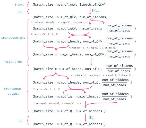
在实现过程中通常选择缩放点积注意力作为每一个注意力头，为了避免计算代价和参数代价的大幅增长设定$p_q = p_k = p_v = p_o / h$

如果将查询、键和值的线性变换的输出数量设置为$p_q h = p_k h = p_v h = p_o$则可以并行计算$h$个头

$p_o$是通过参数num_hiddens指定的

#@save
def transpose_qkv(X, num_heads):
    """为了多注意力头的并行计算而变换形状"""
    # 输入X的形状:(batch_size，seq_len，num_hiddens)
    # 输出X的形状:(batch_size, seq_len, num_heads, head_dim)
    X = X.reshape(X.shape[0], X.shape[1], num_heads, -1)

    # 输出X的形状:(batch_size, num_heads, seq_len, head_dim)
    X = X.permute(0, 2, 1, 3)
    # 因为接下来想把每个 head 当成一个“独立的注意力”在 batch 维度上并行计算

    # 最终输出的形状:(batch_size * num_heads, seq_len, head_dim)
    return X.reshape(-1, X.shape[2], X.shape[3])
    # 把“多头注意力”转化成“一个 batch 里有很多个普通注意力”,就可以用同一个 attention 函数并行算所有头

#@save
def transpose_output(X, num_heads):
    """逆转transpose_qkv函数的操作"""
    # X.shape: (batch_size * num_heads, seq_len, head_dim)
    X = X.reshape(-1, num_heads, X.shape[1], X.shape[2])
    # 把 seq_len 放回中间
    X = X.permute(0, 2, 1, 3)
    # 拼回 num_hiddens  (batch_size, seq_len, num_hiddens)
    return X.reshape(X.shape[0], X.shape[1], -1)

#@save
class MultiHeadAttention(nn.Module):
    """多头注意力"""
    def __init__(self, key_size, query_size, value_size, num_hiddens,
                 num_heads, dropout, bias=False, **kwargs):
        super().__init__(**kwargs)
        self.num_heads = num_heads
        self.attention = d2l.DotProductAttention(dropout)
        # Transformer 的 Q / K / V 不是直接用输入，而是通过线性映射得到的
        self.W_q = nn.Linear(query_size, num_hiddens, bias=bias)
        self.W_k = nn.Linear(key_size, num_hiddens, bias=bias)
        self.W_v = nn.Linear(value_size, num_hiddens, bias=bias)
        # 把拼接后的多头结果，再线性变换一次
        self.W_o = nn.Linear(num_hiddens, num_hiddens, bias=bias)

    def forward(self, queries, keys, values, valid_lens):
        # queries，keys，values: (batch_size, seq_len, num_hiddens)
        # valid_lens:  # (batch_size，)或(batch_size，seq_len)
        # 经过变换后queries，keys，values形状:
        # (batch_size * num_heads, seq_len, head_dim)
        queries = transpose_qkv(self.W_q(queries), self.num_heads)
        keys = transpose_qkv(self.W_k(keys), self.num_heads)
        values = transpose_qkv(self.W_v(values), self.num_heads)

        if valid_lens is not None:
            # 在轴0，将第一项(标量或者矢量)复制num_heads次，
            # 然后如此复制第二项，然后诸如此类。
            valid_lens = torch.repeat_interleave(
                valid_lens, repeats=self.num_heads, dim=0)

        # 多个 head 的点积注意力并行计算
        # output的形状:(batch_size*num_heads，查询的个数，
        # num_hiddens/num_heads)
        output = self.attention(queries, keys, values, valid_lens)

        # 合并多头
        # output_concat: (batch_size, seq_len, num_hiddens)
        output_concat = transpose_output(output, self.num_heads)
        return self.W_o(output_concat)

使用键和值相同的小例子来测试编写的MultiHeadAttention类

多头注意力输出的形状是(batch_size，num_queries，num_hiddens)

num_hiddens, num_heads = 64, 8
attention = MultiHeadAttention(num_hiddens, num_hiddens, num_hiddens,
                               num_hiddens, num_heads, 0.2)
attention.eval()

MultiHeadAttention(
  (attention): DotProductAttention(
    (dropout): Dropout(p=0.2, inplace=False)
  )
  (W_q): Linear(in_features=64, out_features=64, bias=False)
  (W_k): Linear(in_features=64, out_features=64, bias=False)
  (W_v): Linear(in_features=64, out_features=64, bias=False)
  (W_o): Linear(in_features=64, out_features=64, bias=False)
)

batch_size, num_queries = 2, 4
num_kvpairs, valid_lens =  6, torch.tensor([4, 5])
# X = torch.ones((batch_size, num_queries, num_hiddens))
# Y = torch.ones((batch_size, num_kvpairs, num_hiddens))
X = torch.randn((batch_size, num_queries, num_hiddens))
Y = torch.randn((batch_size, num_kvpairs, num_hiddens))
attention(X, Y, Y, valid_lens).shape

torch.Size([2, 4, 64])

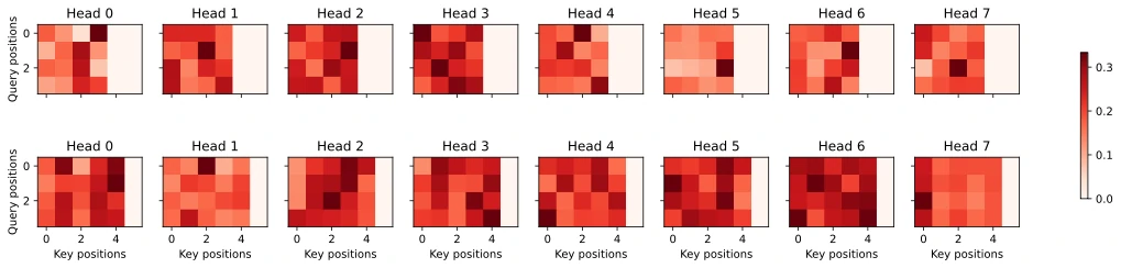
分别可视化这个实验中的多个头的注意力权重

attn_weights = attention.attention.attention_weights  
# reshape之前: (batch_size * num_heads, num_queries, num_kvpairs) torch.Size([16, 4, 6])

attn_weights = attn_weights.reshape(
    batch_size,
    num_heads,
    num_queries,
    num_kvpairs
)

自注意力和位置编码

在深度学习中，经常使用卷积神经网络(CNN)或循环神经网络(RNN)对序列进行编码

有了注意力机制之后，将词元序列输入注意力池化中，以便同一组词元同时充当查询、键和值

每个查询都会关注所有的键－值对并生成一个注意力输出，由于查询、键和值来自同一组输入，因此被称为自注意力(self-attention) ([Lin et al., 2017], [Vaswani et al., 2017])， 也被称为内部注意力(intra-attention) ([Cheng et al., 2016], [Parikh et al., 2016], [Paulus et al., 2017])

自注意力

给定一个由词元组成的输入序列$\mathbf{x}_1, \ldots, \mathbf{x}_n$，其中任意$\mathbf{x}_i \in \mathbb{R}^d$，该序列的自注意力输出为一个长度相同的序列$\mathbf{y}_1, \ldots, \mathbf{y}_n$
$$
\mathbf y_i = f(\mathbf x_i, (\mathbf x_1, \mathbf x_1), \ldots, (\mathbf x_n, \mathbf x_n)) \in \mathbb{R}^d
$$
输出与输入的张量形状相同

num_hiddens, num_heads = 128, 8
attention = d2l.MultiHeadAttention(num_hiddens, num_heads, 0.2)
attention.eval()

MultiHeadAttention(
  (attention): DotProductAttention(
    (dropout): Dropout(p=0.2, inplace=False)
  )
  (W_q): LazyLinear(in_features=0, out_features=128, bias=False)
  (W_k): LazyLinear(in_features=0, out_features=128, bias=False)
  (W_v): LazyLinear(in_features=0, out_features=128, bias=False)
  (W_o): LazyLinear(in_features=0, out_features=128, bias=False)
)

batch_size, num_queries, valid_lens = 2, 4, torch.tensor([4, 5])
X = torch.ones((batch_size, num_queries, num_hiddens))
attention(X, X, X, valid_lens).shape

torch.Size([2, 4, 128])

比较卷积神经网络、循环神经网络和自注意力

比较下面几个架构，目标都是将由$n$个词元组成的序列映射到另一个长度相等的序列，其中的每个输入词元或输出词元都由$d$维向量表示

比较的是卷积神经网络(填充词元被忽略)、循环神经网络和自注意力这几个架构的计算复杂性、顺序操作和最大路径长度

顺序操作会妨碍并行计算，而任意的序列位置组合之间的路径越短，则能更轻松地学习序列中的远距离依赖关系

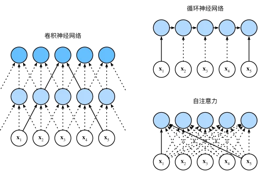
考虑一个卷积核大小为$k$的卷积层，由于序列长度是$n$，输入和输出的通道数量都是$d$，所以卷积层的计算复杂度为$\mathcal{O}(knd^2)$，卷积神经网络是分层的，因此为有$\mathcal{O}(1)$个顺序操作，最大路径长度为$\mathcal{O}(n/k)$

例如$\mathbf{x}_1$和$\mathbf{x}_5$都在卷积核大小为3的双层卷积神经网络的感受野内

当更新循环神经网络的隐状态时$d \times d$权重矩阵和$d$维隐状态的乘法计算复杂度为$\mathcal{O}(d^2)$，由于序列长度是$n$，因此循环神经网络层的计算复杂度为$\mathcal{O}(nd^2)$，有$\mathcal{O}(n)$个顺序操作无法并行化，最大路径长度也是$\mathcal{O}(n)$

在自注意力中，查询、键和值都是$n \times d$矩阵，考虑缩放的”点－积“注意力，其中$n \times d$乘以$d \times n$矩阵，之后输出的$n \times n$矩阵乘以$n \times d$矩阵，因此，自注意力具有$\mathcal{O}(n^2d)$计算复杂性

每个词元都通过自注意力直接连接到任何其他词元，因此有$\mathcal{O}(1)$个顺序操作可以并行计算，最大路径长度也是$\mathcal{O}(1)$

模型	计算复杂度	顺序操作	最大路径
CNN	O(knd²)	O(1)	O(n/k)
RNN	O(nd²)	O(n)	O(n)
Self-Attention	O(n²d)	O(1)	O(1)

总而言之，卷积神经网络和自注意力都拥有并行计算的优势，而且自注意力的最大路径长度最短

但是因为其计算复杂度是关于序列长度的二次方，所以在很长的序列中计算会非常慢

位置编码

在处理词元序列时，循环神经网络是逐个的重复地处理词元的，而自注意力则因为并行计算而放弃了顺序操作

为了使用序列的顺序信息，通过在输入表示中添加**位置编码(positional encoding)**来注入绝对的或相对的位置信息

位置编码可以通过学习得到也可以直接固定得到，接下来描述的是基于正弦函数和余弦函数的固定位置编码(Vaswani et al., 2017)

假设输入表示$\mathbf{X} \in \mathbb{R}^{n \times d}$包含一个序列中$n$个词元的$d$维嵌入表示，位置编码使用相同形状的位置嵌入矩阵$\mathbf{P} \in \mathbb{R}^{n \times d}$输出$\mathbf{X} + \mathbf{P}$，矩阵第$i$行，第$2j$列和$2j+1$列上的元素为：
$$
\begin{split}\begin{aligned} p_{i, 2j} &= \sin\left(\frac{i}{10000^{2j/d}}\right),\\
p_{i, 2j+1} &= \cos\left(\frac{i}{10000^{2j/d}}\right).\end{aligned}\end{split}
$$

#@save
class PositionalEncoding(nn.Module):
    """位置编码"""
    def __init__(self, num_hiddens, dropout, max_len=1000):
        super().__init__()
        self.dropout = nn.Dropout(dropout)
        # 创建一个足够长的P
        # P[0, pos, :] = 第 pos 个位置的编码向量
        self.P = torch.zeros((1, max_len, num_hiddens))
        # .reshape(-1, 1) 所有位置编号，纵着排
        X = torch.arange(max_len, dtype=torch.float32).reshape(-1, 1)
        X = X / torch.pow(
            10000,
            torch.arange(0, num_hiddens, 2) / num_hiddens
        )
        # 偶数维 → 用 sin
        # 奇数维 → 用 cos
        self.P[:, :, 0::2] = torch.sin(X)
        self.P[:, :, 1::2] = torch.cos(X)

    def forward(self, X):
        X = X + self.P[:, :X.shape[1], :].to(X.device)
        return self.dropout(X)

为什么要用 sin / cos？

1️⃣ 连续 & 平滑

• 相邻位置 → 编码差异小
• 远位置 → 编码差异大

2️⃣ 不同维度 = 不同频率

• 低维：变化慢(捕捉长距离)
• 高维：变化快(捕捉局部顺序)

3️⃣ 相对位置信息可线性表示：对于任意偏移 k，PE(pos + k) 可以用 PE(pos) 的线性变换表示

不同batch相同位置+相同的位置编码，位置编码不会盖住词向量，只是一个bias，模型后续看到的是“词 + 位置信息的混合体”

顺序信息是怎么“浮现”的？

不同位置有不同PE，即使词相同，只要位置不同$q_i ≠ q_{i+1}$，于是注意力矩阵里得到的 score 不同，相当于间接看见了顺序

在位置嵌入矩阵$\mathbf{P}$中，行代表词元在序列中的位置，列代表位置编码的不同维度

从下面的例子中可以看到位置嵌入矩阵的第6列和第7列的频率高于第8列和第9列，第6列和第7列之间的偏移量(第8列和第9列相同)是由于正弦函数和余弦函数的交替

encoding_dim, num_steps = 32, 60
pos_encoding = PositionalEncoding(encoding_dim, 0)
pos_encoding.eval()
X = pos_encoding(torch.zeros((1, num_steps, encoding_dim)))
P = pos_encoding.P[:, :X.shape[1], :]
d2l.plot(torch.arange(num_steps), P[0, :, 6:10].T, xlabel='Row (position)',
         figsize=(6, 2.5), legend=["Col %d" % d for d in torch.arange(6, 10)])

绝对位置信息

在二进制表示中，较高比特位的交替频率低于较低比特位

正余弦位置编码，用“不同频率的连续信号”，模拟了二进制中“高位慢变、低位快变”的层级结构，维度越靠后，对应的 sin/cos 频率越低

由于输出是浮点数，因此此类连续表示比二进制表示法更节省空间

P = P[0, :, :].unsqueeze(0).unsqueeze(0)
d2l.show_heatmaps(P, xlabel='Column (encoding dimension)',
                  ylabel='Row (position)', figsize=(3.5, 4), cmap='Blues')

---

用 d=4 的位置编码，手算 pos=0,1,2 的完整行，这里假设max_len为10000
$$
\begin{aligned}
P E(p o s, 2 i) & =\sin \left(\frac{p o s}{10000^{2 i / d}}\right) \\
P E(p o s, 2 i+1) & =\cos \left(\frac{p o s}{10000^{2 i / d}}\right)
\end{aligned}
$$
$d = 4$，那么维度索引：0, 1, 2, 3，所以 $i$ 只能取 0 和 1

对于$i=0$，分母为1，对于$i=1$，分母为100

pos = 0:

PE(0) ≈
[
  0, # sin(0)
  1, # cos(0)
  0, # sin(1)
  1  # cos(1)
]

pos = 1：

PE(1) ≈
[
  0.8415, # sin(1)
  0.5403, # cos(1)
  0.0100, # sin(1/100)
  0.9999  # cos(1/100)
]

pos = 2：

PE(2) ≈
[
  0.9093,  # sin(2)
 -0.4161,  # cos(2)
  0.0200,  # sin(2/100)
  0.9998   # cos(2/100)
]

相对位置信息

除了捕获绝对位置信息之外，上述的位置编码还允许模型学习得到输入序列中相对位置信息

这是因为对于任何确定的位置偏移$\delta$，位置$i + \delta$处的位置编码可以线性投影位置$i$处的位置编码来表示

Transformer

Transformer模型完全基于注意力机制，没有任何卷积层或循环神经网络层

尽管Transformer最初是应用于在文本数据上的序列到序列学习，但现在已经推广到各种现代的深度学习中，例如语言、视觉、语音和强化学习领域

模型

Transformer是由编码器和解码器组成的，与基于Bahdanau注意力实现的序列到序列的学习相比，Transformer的编码器和解码器是基于自注意力的模块叠加而成的，源(输入)序列和目标(输出)序列的嵌入(embedding)表示将加上位置编码(positional encoding)，再分别输入到编码器和解码器中

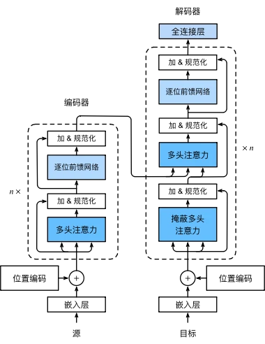
Transformer 的编码器由多个结构完全相同的层堆叠而成，每一层包含两个子层

1. 多头自注意力(Multi-Head Self-Attention)

   查询(Query)、键(Key)、值(Value)均来自前一编码器层的输出，用于建模序列中不同位置之间的全局依赖关系

2. 基于位置的前馈网络(Position-wise Feed-Forward Network)

   对每个位置的向量独立进行非线性变换，不同位置共享参数

每个子层都采用残差连接(residual connection)和层规范化(layer normalization)

对于序列中任何位置的任何输入$\mathbf{x} \in \mathbb{R}^d$，都要求满足$\mathrm{sublayer}(\mathbf{x}) \in \mathbb{R}^d$，以便满足残差连接

输入序列中每个位置，编码器最终都会输出一个$d$维的上下文相关表示向量

解码器同样由多个相同的层堆叠而成，并且同样使用残差连接和层规范化

1. 掩蔽多头自注意力(Masked Multi-Head Self-Attention)

   只允许当前位置关注之前的位置，通过 mask 阻止“看到未来信息，保证模型具有自回归(auto-regressive)属性

2. 编码器－解码器注意力(Encoder-Decoder Attention)

   Query：来自前一解码器层的输出；Key / Value：来自整个编码器的输出

   用于在生成过程中选择性关注输入序列的相关部分

3. FFN结构和编码器相同

对比维度	编码器（Encoder）	解码器（Decoder）
主要功能	理解输入序列	生成输出序列
是否自回归	否	是
自注意力	无 mask，可看全序列	有 mask，只看过去
输入来源	原始输入序列	已生成的输出 + 编码器输出
输出作用	提供语义表示	逐步预测下一个词元

基于位置的前馈网络

基于位置的前馈网络对序列中的所有位置的表示进行变换时使用的是同一个多层感知机(MLP)，这就是称前馈网络是基于位置的(positionwise)的原因

输入X的形状(batch_size，seq_len，d_model)将被一个两层的感知机转换成形状为(batch_size，seq_len，ffn_num_outputs)的输出张量

#@save
class PositionWiseFFN(nn.Module):
    """基于位置的前馈网络"""
    def __init__(self, ffn_num_input, ffn_num_hiddens, ffn_num_outputs,
                 **kwargs):
        super().__init__(**kwargs)
        self.dense1 = nn.Linear(ffn_num_input, ffn_num_hiddens)
        self.relu = nn.ReLU()
        self.dense2 = nn.Linear(ffn_num_hiddens, ffn_num_outputs)

    def forward(self, X):
        return self.dense2(self.relu(self.dense1(X)))

因为用同一个多层感知机对所有位置上的输入进行变换，所以当所有这些位置的输入相同时，它们的输出也是相同的

ffn = PositionWiseFFN(4, 4, 8)
ffn.eval()
ffn(torch.ones((2, 3, 4)))[0]

tensor([[ 0.5157,  0.2434,  0.4663, -0.0975,  0.1334, -0.3209, -0.1155, -0.5577],
        [ 0.5157,  0.2434,  0.4663, -0.0975,  0.1334, -0.3209, -0.1155, -0.5577],
        [ 0.5157,  0.2434,  0.4663, -0.0975,  0.1334, -0.3209, -0.1155, -0.5577]],
       grad_fn=<SelectBackward0>)

残差连接和层规范化

层规范化和批量规范化的目标相同，但层规范化是基于特征维度进行规范化

尽管批量规范化在计算机视觉中被广泛应用，但在自然语言处理任务中(输入通常是变长序列)批量规范化通常不如层规范化的效果好

BN：跨 batch 统计的规范化

[B, C, L]  或  [B, C, H, W]

对每一个通道 C，在整个 batch(以及空间维度)上计算均值和方差

BN假设：同一个 batch 中，不同样本在统计意义上是“可比的”

LN：单个样本内部的规范化

只在当前样本内部，对所有特征维度计算均值和方差

LN假设：一个 token / 一个时间步的各个特征维度之间是可比的

	BatchNorm	LayerNorm
统计范围	batch 内多个样本	单个样本
是否依赖 batch size	强烈依赖	完全不依赖
是否受序列长度影响	会	不会
适合任务	图像	NLP / Transformer

可以使用残差连接和层规范化来实现AddNorm类，暂退法也被作为正则化方法使用

#@save
class AddNorm(nn.Module):
    """残差连接后进行层规范化"""
    def __init__(self, normalized_shape, dropout, **kwargs):
        super().__init__(**kwargs)
        self.dropout = nn.Dropout(dropout)
        self.ln = nn.LayerNorm(normalized_shape)

    def forward(self, X, Y):
        return self.ln(self.dropout(Y) + X)

编码器

有了组成Transformer编码器的基础组件，现在可以先实现编码器中的一个层

EncoderBlock类包含两个子层：多头自注意力和基于位置的前馈网络，这两个子层都使用了残差连接和紧随的层规范化

#@save
class EncoderBlock(nn.Module):
    """Transformer编码器块"""
    def __init__(self, num_hiddens, norm_shape, ffn_num_input,
                 ffn_num_hiddens, num_heads,
                 dropout, use_bias=False, **kwargs):
        super().__init__(**kwargs)
        self.attention = d2l.MultiHeadAttention(
            num_hiddens, num_heads, dropout, use_bias)
        self.addnorm1 = AddNorm(norm_shape, dropout)
        self.ffn = PositionWiseFFN(
            ffn_num_input, ffn_num_hiddens, num_hiddens)
        self.addnorm2 = AddNorm(norm_shape, dropout)

    def forward(self, X, valid_lens):
        Y = self.addnorm1(X, self.attention(X, X, X, valid_lens))
        return self.addnorm2(Y, self.ffn(Y))

Transformer编码器中的任何层都不会改变其输入的形状

下面实现的Transformer编码器的代码中，堆叠了num_layers个EncoderBlock类的实例

这里使用的是值范围在-1和1之间的固定位置编码，因此通过学习得到的输入的嵌入表示的值需要先乘以嵌入维度的平方根进行重新缩放，然后再与位置编码相加

#@save
class TransformerEncoder(d2l.Encoder):
    """Transformer编码器"""
    def __init__(self, vocab_size, num_hiddens, norm_shape,
                 ffn_num_input, ffn_num_hiddens,
                 num_heads, num_layers, dropout, use_bias=False, **kwargs):
        super().__init__(**kwargs)
        self.num_hiddens = num_hiddens
        self.embedding = nn.Embedding(vocab_size, num_hiddens)
        self.pos_encoding = d2l.PositionalEncoding(num_hiddens, dropout)
        self.blks = nn.Sequential()
        for i in range(num_layers):
            self.blks.add_module("block"+str(i),
                EncoderBlock(num_hiddens, norm_shape, ffn_num_input,
                             ffn_num_hiddens,
                             num_heads, dropout, use_bias))

    def forward(self, X, valid_lens, *args):
        # 因为位置编码值在-1和1之间，
        # 因此嵌入值乘以嵌入维度的平方根进行缩放，
        # 然后再与位置编码相加。
        X = self.pos_encoding(self.embedding(X) * math.sqrt(self.num_hiddens))
        self.attention_weights = [None] * len(self.blks)
        for i, blk in enumerate(self.blks):
            X = blk(X, valid_lens)
            self.attention_weights[
                i] = blk.attention.attention.attention_weights
        return X

指定了超参数来创建一个两层的Transformer编码器，输出的形状是(批量大小，时间步数目，num_hiddens)

encoder = TransformerEncoder(
    vocab_size=100,
    num_hiddens=24,
    norm_shape=24,
    ffn_num_input=24,
    ffn_num_hiddens=48,
    num_heads=4,
    num_layers=2,
    dropout=0.5
)
encoder.eval()
encoder(torch.ones((2, 100), dtype=torch.long), valid_lens).shape

torch.Size([2, 100, 24])

解码器

Transformer解码器也是由多个相同的层组成，在DecoderBlock类中实现的每个层包含了三个子层：解码器自注意力、“编码器-解码器”注意力和基于位置的前馈网络

为了在解码器中保留自回归的属性，其掩蔽自注意力设定了参数dec_valid_lens，以便任何查询都只会与解码器中所有已经生成词元的位置(即直到该查询位置为止)进行注意力计算

class DecoderBlock(nn.Module):
    """解码器中第i个块"""
    def __init__(self, num_hiddens, norm_shape, ffn_num_input,
                 ffn_num_hiddens, num_heads,
                 dropout, i, **kwargs):
        super().__init__(**kwargs)
        self.i = i
        self.attention1 = d2l.MultiHeadAttention(
            num_hiddens, num_heads, dropout)
        self.addnorm1 = AddNorm(norm_shape, dropout)
        self.attention2 = d2l.MultiHeadAttention(
            num_hiddens, num_heads, dropout)
        self.addnorm2 = AddNorm(norm_shape, dropout)
        self.ffn = PositionWiseFFN(ffn_num_input, ffn_num_hiddens,
                                   num_hiddens)
        self.addnorm3 = AddNorm(norm_shape, dropout)

    def forward(self, X, state):
        enc_outputs, enc_valid_lens = state[0], state[1]
        # 训练阶段，输出序列的所有词元都在同一时间处理，
        # 因此state[2][self.i]初始化为None。
        # 预测阶段，输出序列是通过词元一个接着一个解码的，
        # 因此state[2][self.i]包含着直到当前时间步第i个块解码的输出表示
        if state[2][self.i] is None:
            key_values = X
        else:
            key_values = torch.cat((state[2][self.i], X), axis=1)
        state[2][self.i] = key_values
        if self.training:
            batch_size, num_steps, _ = X.shape
            # dec_valid_lens的开头:(batch_size,num_steps),
            # 其中每一行是[1,2,...,num_steps]
            dec_valid_lens = torch.arange(
                1, num_steps + 1, device=X.device).repeat(batch_size, 1)
        else:
            dec_valid_lens = None

        # 自注意力
        X2 = self.attention1(X, key_values, key_values, dec_valid_lens)
        Y = self.addnorm1(X, X2)
        # 编码器－解码器注意力。
        # enc_outputs的开头:(batch_size,num_steps,num_hiddens)
        Y2 = self.attention2(Y, enc_outputs, enc_outputs, enc_valid_lens)
        Z = self.addnorm2(Y, Y2)
        return self.addnorm3(Z, self.ffn(Z)), state

假设：生成一句话 y1 y2 y3

t = 1

# 输入
X = [y1]
state[2][i] = None
# 执行
key_values = X  # [y1]
state[2][i] = [y1]

t = 2

# 输入
X = [y2]
state[2][i] = [y1]
# 执行
key_values = torch.cat(([y1], [y2]), dim=1)
state[2][i] = [y1, y2]

t = 3

# 输入
X = [y3]
state[2][i] = [y1, y2]
# 执行
key_values = [y1, y2, y3]
state[2][i] = [y1, y2, y3]

state[2][self.i] = 当前 DecoderBlock 在“到目前为止”已经生成的所有 token 表示

decoder_blk = DecoderBlock(
    num_hiddens=24,
    norm_shape=24,
    ffn_num_input=24,
    ffn_num_hiddens=48,
    num_heads=8,
    dropout=0.5,
    i = 0
)
decoder_blk.eval()
X = torch.ones((2, 100, 24))
state = [encoder_blk(X, valid_lens), valid_lens, [None]]
decoder_blk(X, state)[0].shape

torch.Size([2, 100, 24])

现在构建了由num_layers个DecoderBlock实例组成的完整的Transformer解码器，最后通过一个全连接层计算所有vocab_size个可能的输出词元的预测值。解码器的自注意力权重和编码器解码器注意力权重都被存储下来，方便日后可视化的需要

class TransformerDecoder(d2l.AttentionDecoder):
    def __init__(self, vocab_size, num_hiddens, norm_shape, 
                 ffn_num_input, ffn_num_hiddens,
                 num_heads, num_layers, dropout, **kwargs):
        super(TransformerDecoder, self).__init__(**kwargs)
        self.num_hiddens = num_hiddens
        self.num_layers = num_layers
        self.embedding = nn.Embedding(vocab_size, num_hiddens)
        self.pos_encoding = d2l.PositionalEncoding(num_hiddens, dropout)
        self.blks = nn.Sequential()
        for i in range(num_layers):
            self.blks.add_module("block"+str(i),
                DecoderBlock(num_hiddens,
                             norm_shape, ffn_num_input, ffn_num_hiddens,
                             num_heads, dropout, i))
        self.dense = nn.Linear(num_hiddens, vocab_size)

    def init_state(self, enc_outputs, enc_valid_lens, *args):
        return [enc_outputs, enc_valid_lens, [None] * self.num_layers]

    def forward(self, X, state):
        X = self.pos_encoding(self.embedding(X) * math.sqrt(self.num_hiddens))
        self._attention_weights = [[None] * len(self.blks) for _ in range (2)]
        for i, blk in enumerate(self.blks):
            X, state = blk(X, state)
            # 解码器自注意力权重
            self._attention_weights[0][
                i] = blk.attention1.attention.attention_weights
            # “编码器－解码器”自注意力权重
            self._attention_weights[1][
                i] = blk.attention2.attention.attention_weights
        return self.dense(X), state

    @property
    def attention_weights(self):
        return self._attention_weights

训练

指定Transformer的编码器和解码器都是2层，都使用4头注意力

为了进行序列到序列的学习，下面在“英语－法语”机器翻译数据集上训练Transformer模型

num_hiddens, num_layers, dropout, batch_size, num_steps = 32, 2, 0.1, 64, 10
lr, num_epochs, device = 0.005, 200, d2l.try_gpu()
ffn_num_input, ffn_num_hiddens, num_heads = 32, 64, 4
norm_shape = [32]

train_iter, src_vocab, tgt_vocab = d2l.load_data_nmt(batch_size, num_steps)

encoder = TransformerEncoder(
    len(src_vocab), num_hiddens,
    norm_shape, ffn_num_input, ffn_num_hiddens, num_heads,
    num_layers, dropout)
decoder = TransformerDecoder(
    len(tgt_vocab), num_hiddens,
    norm_shape, ffn_num_input, ffn_num_hiddens, num_heads,
    num_layers, dropout)
net = EncoderDecoderCompat(encoder, decoder)
d2l.train_seq2seq(net, train_iter, lr, num_epochs, tgt_vocab, device)

loss 0.029, 8776.3 tokens/sec on cpu

训练结束后，使用Transformer模型将一些英语句子翻译成法语，并且计算它们的BLEU分数

engs = ['go .', "i lost .", 'he\'s calm .', 'i\'m home .']
fras = ['va !', 'j\'ai perdu .', 'il est calme .', 'je suis chez moi .']
for eng, fra in zip(engs, fras):
    translation, dec_attention_weight_seq = d2l.predict_seq2seq(
        net, eng, src_vocab, tgt_vocab, num_steps, device, True)
    print(f'{eng} => {translation}, ',
          f'bleu {d2l.bleu(translation, fra, k=2):.3f}')

go . => va !,  bleu 1.000
i lost . => j'ai perdu .,  bleu 1.000
he's calm . => il est calme .,  bleu 1.000
i'm home . => je suis chez moi .,  bleu 1.000

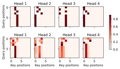
当进行最后一个英语到法语的句子翻译工作时，可视化Transformer的注意力权重

编码器自注意力权重的形状为(编码器层数，注意力头数，num_steps或查询的数目，num_steps或“键－值”对的数目)

d2l.show_heatmaps(
    enc_attention_weights.cpu(), xlabel='Key positions',
    ylabel='Query positions', titles=['Head %d' % i for i in range(1, 5)],
    figsize=(7, 3.5))

逐行呈现两层多头注意力的权重，每个注意力头都根据查询、键和值的不同的表示子空间来表示不同的注意力