图像增广 在卷积神经网络提到大型数据集是成功应用深度神经网络的先决条件
图像增广在对训练图像进行一系列的随机变化之后,生成相似但不同的训练样本,从而扩大了训练集的规模
应用图像增广的原因是,随机改变训练样本可以减少模型对某些属性的依赖,从而提高模型的泛化能力,例如可以以不同的方式裁剪图像,使感兴趣的对象出现在不同的位置,减少模型对于对象出现位置的依赖;还可以调整亮度、颜色等因素来降低模型对颜色的敏感度
图像增广技术对于AlexNet的成功是必不可少的
1
2
3
4
5
6
7
8
import torchimport torchvision from torchvision import transforms from torchvision import datasets from torch.utils import data from torch import nnimport matplotlib.pyplot as pltfrom PIL import Image
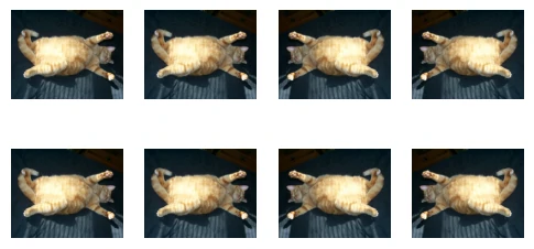
常用方法 在对常用图像增广方法的探索时,将使用下面这个尺寸为400×500的图像作为示例
1
2
3
4
img = Image.open ('imgs/cat1.jpg' ) plt.imshow(img) plt.axis('off' ) plt.show()
大多数图像增广方法都具有一定的随机性
定义辅助函数apply,此函数在输入图像img上多次运行图像增广方法aug并显示所有结果
1
2
3
4
5
6
7
8
9
10
11
12
13
14
15
16
17
18
19
def show_images (imgs, num_rows, num_cols, titles=None , scale=1.5 ): """Plot a list of images.""" figsize = (num_cols * scale, num_rows * scale) _, axes = plt.subplots(num_rows, num_cols, figsize=figsize) axes = axes.flatten() for i, (ax, img) in enumerate (zip (axes, imgs)): if torch.is_tensor(img): img = img.detach().numpy() ax.imshow(img) ax.axis('off' ) if titles: ax.set_title(titles[i]) plt.show() def apply (img, aug, num_rows=2 , num_cols=4 , scale=1.5 ): Y = [aug(img) for _ in range (num_rows * num_cols)] show_images(Y, num_rows, num_cols, scale=scale)
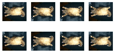
翻转和裁剪 左右翻转图像通常不会改变对象的类别,这是最早且最广泛使用的图像增广方法之一
使用transforms模块来创建RandomFlipLeftRight实例,这样就各有50%的几率使图像向左或向右翻转
1 apply(img, transforms.RandomHorizontalFlip())
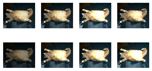
上下翻转图像不如左右图像翻转那样常用,至少对于这个图像,上下翻转不会妨碍识别
创建一个RandomFlipTopBottom实例,使图像各有50%的几率向上或向下翻转
1 apply(img, transforms.RandomVerticalFlip())
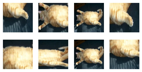
示例图片中猫位于图片的中间,但并非所有图片都是这样,汇聚层可以降低卷积层对目标位置的敏感性,另外也可以通过对图像进行随机裁剪,使物体以不同的比例出现在图像的不同位置,也可以降低模型对目标位置的敏感性
随机裁剪的区域面积占原始面积的10%到100%,该区域的宽高比从0.5~2之间随机取值,然后区域的宽度和高度都被缩放到200像素
正常都是取均匀分布,除非另外说明
1
2
3
shape_aug = transforms.RandomResizedCrop( (200 , 200 ), scale=(0.1 , 1 ), ratio=(0.5 , 2 )) apply(img, shape_aug)
改变颜色 另一种增广方法是改变颜色,可以改变图像颜色的四个方面:亮度、对比度、饱和度和色相
在下面的代码中随机更改图像的亮度,随机值为原始图像的50%-150%
1
2
3
4
5
apply(img, transforms.ColorJitter( brightness=0.5 , contrast=0 , saturation=0 , hue=0 ))
但是一般都是处理灰度图片,所以主要调整亮度
如果同时更改
1
2
3
color_aug = transforms.ColorJitter( brightness=0.5 , contrast=0.5 , saturation=0.5 , hue=0.5 ) apply(img, color_aug)
综合使用 在实践中将结合多种图像增广方法,可以通过使用一个Compose实例来综合上面定义的不同的图像增广方法,并将它们应用到每个图像
1
2
3
4
5
augs = transforms.Compose([ transforms.RandomHorizontalFlip(), color_aug, shape_aug]) apply(img, augs)
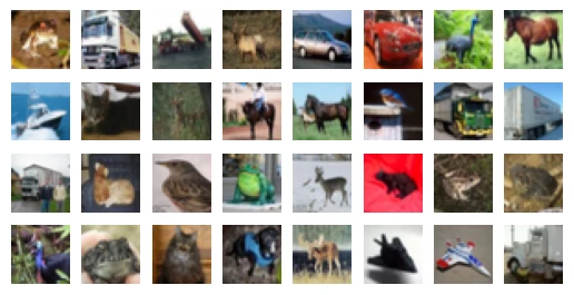
训练 使用图像增广来训练模型,这里使用CIFAR-10数据集,而不是之前使用的Fashion-MNIST数据集,这是因为Fashion-MNIST数据集中对象的位置和大小已被规范化,而CIFAR-10数据集中对象的颜色和大小差异更明显
1
2
all_images = datasets.CIFAR10(root="../data" , train=True , download=True ) show_images([all_images[i][0 ] for i in range (32 )], 4 , 8 , scale=0.8 );
为了保证预测结果稳定,只在训练阶段使用图像增广,预测时不进行随机增广操作
在这里只使用最简单的随机左右翻转,使用ToTensor实例将一批图像转换为深度学习框架所要求的格式,即形状为(批量大小,通道数,高度,宽度)的32位浮点数,取值范围为0~1
1
2
3
4
5
6
train_augs = transforms.Compose([ transforms.RandomHorizontalFlip(), transforms.ToTensor()]) test_augs = transforms.Compose([ transforms.ToTensor()])
定义一个辅助函数,以便于读取图像和应用图像增广
PyTorch数据集提供的transform参数应用图像增广来转化图像
1
2
3
4
5
6
7
8
9
10
def load_cifar10 (is_train, augs, batch_size ): dataset = datasets.CIFAR10( root="../data" , train=is_train, transform=augs, download=True ) dataloader = data.DataLoader(dataset, batch_size=batch_size, shuffle=is_train, num_workers=get_dataloader_workers()) return dataloader
data.DataLoader:
dataset:加载的数据集batch_size:每次从数据集中取多少个样本组成一个 batchshuffle:是否在每个 epoch 开始前随机打乱数据,训练一般Truenum_workers:并行加载数据的子进程数
多GPU训练 在CIFAR-10数据集上训练ResNet-18模型,需要利用多GPU实现
1 2 3 4 5 6 7 8 9 10 11 12 13 14 15 16 17 18 19 20 21 22 23 24 25 26 27 28 29 30 31 32 33 34 35 36 37 38 39 40 41 42 43 44 45 46 47 def train_batch_ch13 (net, X, y, loss, trainer, devices ): """用多GPU进行小批量训练""" if isinstance (X, list ): X = [x.to(devices[0 ]) for x in X] else : X = X.to(devices[0 ]) y = y.to(devices[0 ]) net.train() trainer.zero_grad() pred = net(X) l = loss(pred, y) l.sum ().backward() trainer.step() train_loss_sum = l.sum () train_acc_sum = accuracy(pred, y) return train_loss_sum, train_acc_sum def train_ch13 (net, train_iter, test_iter, loss, trainer, num_epochs, devices=try_all_gpus( ): """用多GPU进行模型训练""" timer, num_batches = Timer(), len (train_iter) animator = Animator(xlabel='epoch' , xlim=[1 , num_epochs], ylim=[0 , 1 ], legend=['train loss' , 'train acc' , 'test acc' ]) net = nn.DataParallel(net, device_ids=devices).to(devices[0 ]) for epoch in range (num_epochs): metric = Accumulator(4 ) for i, (features, labels) in enumerate (train_iter): timer.start() l, acc = train_batch_ch13( net, features, labels, loss, trainer, devices) metric.add(l, acc, labels.shape[0 ], labels.numel()) timer.stop() if (i + 1 ) % (num_batches // 5 ) == 0 or i == num_batches - 1 : animator.add(epoch + (i + 1 ) / num_batches, (metric[0 ] / metric[2 ], metric[1 ] / metric[3 ], None )) test_acc = evaluate_accuracy_gpu(net, test_iter) animator.add(epoch + 1 , (None , None , test_acc)) animator.show() print (f'loss {metric[0 ] / metric[2 ]:.3 f} , train acc ' f'{metric[1 ] / metric[3 ]:.3 f} , test acc {test_acc:.3 f} ' ) print (f'{metric[2 ] * num_epochs / timer.sum ():.1 f} examples/sec on ' f'{str (devices)} ' )
自定义resnet18网络,把第一层改为3×3卷积层,因为cifar10的图片不是224,也是32×32,如果保持7×7会出问题,而且减少了第一组的池化层
1 2 3 4 5 6 7 8 9 10 11 12 13 14 15 16 17 18 19 20 21 22 23 24 25 26 27 28 29 30 31 32 33 34 35 36 37 38 39 40 41 42 43 44 45 46 47 48 49 50 51 52 53 54 55 class Residual (nn.Module): def __init__ (self, in_channels, out_channels, use_1x1conv=False , stride=1 ): super ().__init__() self .conv1 = nn.Conv2d(in_channels, out_channels, kernel_size=3 , padding=1 , stride=stride) self .conv2 = nn.Conv2d(out_channels, out_channels, kernel_size=3 , padding=1 ) if use_1x1conv: self .conv3 = nn.Conv2d(in_channels, out_channels, kernel_size=1 , stride=stride) else : self .conv3 = None self .bn1 = nn.BatchNorm2d(out_channels) self .bn2 = nn.BatchNorm2d(out_channels) def forward (self, X ): Y = nn.functional.relu(self .bn1(self .conv1(X))) Y = self .bn2(self .conv2(Y)) if self .conv3: X = self .conv3(X) Y += X return nn.functional.relu(Y) def resnet_block (in_channels, out_channels, num_residuals, first_block=False ): blk = [] for i in range (num_residuals): if i == 0 and not first_block: blk.append(Residual(in_channels, out_channels, use_1x1conv=True , stride=2 )) else : blk.append(Residual(out_channels, out_channels)) return blk def resnet18 (num_classes, in_channels=3 ): net = nn.Sequential( nn.Conv2d(in_channels, 64 , kernel_size=3 , stride=1 , padding=3 ), nn.BatchNorm2d(64 ), nn.ReLU() ) net.add_module("resnet_block1" , nn.Sequential(*resnet_block(64 , 64 , 2 , first_block=True ))) net.add_module("resnet_block2" , nn.Sequential(*resnet_block(64 , 128 , 2 ))) net.add_module("resnet_block3" , nn.Sequential(*resnet_block(128 , 256 , 2 ))) net.add_module("resnet_block4" , nn.Sequential(*resnet_block(256 , 512 , 2 ))) net.add_module("global_avg_pool" , nn.AdaptiveAvgPool2d((1 , 1 ))) net.add_module("fc" , nn.Sequential(nn.Flatten(), nn.Linear(512 , num_classes))) return net
可以定义train_with_data_aug函数,使用图像增广来训练模型
该函数获取所有的GPU,并使用Adam作为训练的优化算法,将图像增广应用于训练集,最后调用刚刚定义的用于训练和评估模型的train_ch13函数
1 2 3 4 5 6 7 8 9 10 11 12 13 14 15 16 17 18 19 batch_size, devices, net = 256 , try_all_gpus(), resnet18(10 , 3 ) def init_weights (m ): if type (m) in [nn.Linear, nn.Conv2d]: nn.init.xavier_uniform_(m.weight) net.apply(init_weights) def train_with_data_aug (train_augs, test_augs, net, lr=0.001 ): train_iter = load_cifar10(True , train_augs, batch_size) test_iter = load_cifar10(False , test_augs, batch_size) loss = nn.CrossEntropyLoss(reduction="none" ) trainer = torch.optim.Adam(net.parameters(), lr=lr) train_ch13(net, train_iter, test_iter, loss, trainer, 10 , devices)
1
2
3
4
5
6
7
8
9
10
epoch 1, loss 1.427, acc 0.490, test acc 0.498, time 82.98 sec epoch 2, loss 0.884, acc 0.687, test acc 0.517, time 83.32 sec epoch 3, loss 0.659, acc 0.770, test acc 0.675, time 82.61 sec epoch 4, loss 0.524, acc 0.818, test acc 0.758, time 83.24 sec epoch 5, loss 0.430, acc 0.851, test acc 0.767, time 82.97 sec epoch 6, loss 0.360, acc 0.875, test acc 0.805, time 83.55 sec epoch 7, loss 0.307, acc 0.893, test acc 0.819, time 83.18 sec epoch 8, loss 0.258, acc 0.910, test acc 0.838, time 83.17 sec epoch 9, loss 0.217, acc 0.926, test acc 0.844, time 82.58 sec epoch 10, loss 0.186, acc 0.936, test acc 0.851, time 81.58 sec
1
2
loss 0.186, train acc 0.936, test acc 0.851 1383.1 examples/sec on [device(type='cuda', index=0)]
这里仅使用随机左右翻转的图像增广来训练模型
小结
图像增广基于现有的训练数据生成随机图像,来提高模型的泛化能力
为了在预测过程中得到确切的结果,通常对训练样本只进行图像增广,而在预测过程中不使用带随机操作的图像增广
深度学习框架提供了许多不同的图像增广方法,这些方法可以被同时应用
微调 由于训练样本数量有限,训练模型的准确性可能无法满足实际要求
另一种解决方案是应用**迁移学习(transfer learning)**将从源数据集学到的知识迁移到目标数据集,尽管ImageNet数据集中的大多数图像与椅子无关,但在此数据集上训练的模型可能会提取更通用的图像特征,这有助于识别边缘、纹理、形状和对象组合,这些类似的特征也可能有效地识别椅子
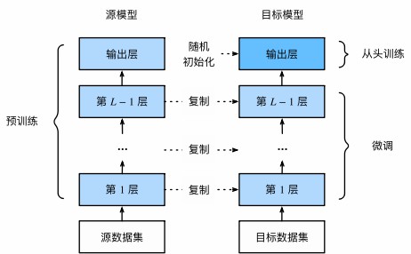
步骤 迁移学习中的常见技巧:微调(fine-tuning)
包括以下四个步骤:
在源数据集(例如ImageNet数据集)上预训练神经网络模型,即源模型
创建一个新的神经网络模型,即目标模型,这将复制源模型上的所有模型设计及其参数(不包括输出层)。前面层的参数包含通用特征,可直接用于新任务;输出层与旧任务标签相关,因此需重新训练
向目标模型添加输出层,其输出数是目标数据集中的类别数,然后随机初始化该层的模型参数
在目标数据集上训练目标模型,输出层将从头开始进行训练,而所有其他层的参数将根据源模型的参数进行微调
当目标数据集比源数据集小得多时,微调有助于提高模型的泛化能力
热狗识别 在一个小型数据集上微调ResNet模型,该模型已在ImageNet数据集上进行了预训练。小型数据集包含数千张包含热狗和不包含热狗的图像,使用微调模型来识别图像中是否包含热狗
获取数据集 使用的热狗数据集来源于网络,该数据集包含1400张热狗的“正类”图像,以及包含尽可能多的其他食物的“负类”图像,含着两个类别的1000张图片用于训练,其余的则用于测试
解压下载的数据集,获得了两个文件夹hotdog/train和hotdog/test,这两个文件夹都有hotdog(有热狗)和not-hotdog(无热狗)两个子文件夹,子文件夹内都包含相应类的图像
1
2
3
4
5
6
DATA_HUB = dict () DATA_URL = 'http://d2l-data.s3-accelerate.amazonaws.com/' DATA_HUB['hotdog' ] = ( DATA_URL + 'hotdog.zip' , 'fba480ffa8aa7e0febbb511d181409f899b9baa5' ) data_dir = download_extract('hotdog' )
创建两个实例来分别读取训练和测试数据集中的所有图像文件
1
2
train_imgs = datasets.ImageFolder(os.path.join(data_dir, 'train' )) test_imgs = datasets.ImageFolder(os.path.join(data_dir, 'test' ))
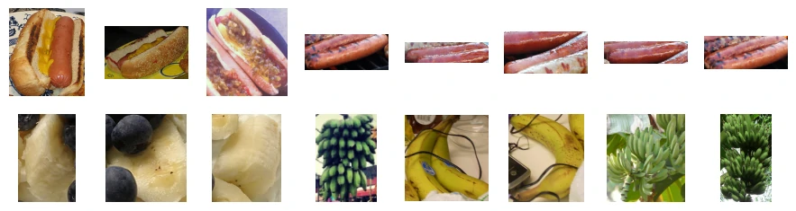
显示前8个正类样本图片和最后8张负类样本图片,图像的大小和纵横比各有不同
1
2
3
hotdogs = [train_imgs[i][0 ] for i in range (8 )] not_hotdogs = [train_imgs[-i - 1 ][0 ] for i in range (8 )] show_images(hotdogs + not_hotdogs, 2 , 8 , scale=1.4 );
输入图像用源模型(预训练模型)原始数据集的均值和标准差来做标准化
1
2
3
4
5
normalize = torchvision.transforms.Normalize( [0.485 , 0.456 , 0.406 ], [0.229 , 0.224 , 0.225 ] )
在训练期间,首先从图像中裁切随机大小和随机长宽比的区域,然后将该区域缩放为224×224的输入图像,再进行随机水平翻转和标准化
1
2
3
4
5
6
7
8
9
train_augs = torchvision.transforms.Compose([ torchvision.transforms.RandomResizedCrop(224 ), torchvision.transforms.RandomHorizontalFlip(), torchvision.transforms.ToTensor(), normalize])
在测试过程中将图像的高度和宽度都缩放到256像素,然后裁剪中央224×224区域作为输入
1
2
3
4
5
6
7
8
9
test_augs = torchvision.transforms.Compose([ torchvision.transforms.Resize([256 , 256 ]), torchvision.transforms.CenterCrop(224 ), torchvision.transforms.ToTensor(), normalize])
定义和初始化模型 使用在ImageNet数据集上预训练的ResNet-18作为源模型,在这里指定pretrained=True以自动下载预训练的模型参数
1 pretrained_net = torchvision.models.resnet18(pretrained=True )
预训练的源模型实例包含许多特征层和一个输出层fc,此划分的主要目的是促进对除输出层以外所有层的模型参数进行微调,下面给出了源模型的成员变量fc
1 Linear(in_features=512, out_features=1000, bias=True)
在ResNet的全局平均池化层后,原来的全连接层输出1000个ImageNet类
构建目标模型时,结构与预训练模型相同,只将输出层改为目标数据集的类别数,目标模型的特征层参数继承自预训练模型,只需用较小学习率微调
输出层参数随机初始化,需要更大学习率(约为特征层的10倍)来从头训练
1
2
3
finetune_net = torchvision.models.resnet18(pretrained=True ) finetune_net.fc = nn.Linear(finetune_net.fc.in_features, 2 ) nn.init.xavier_uniform_(finetune_net.fc.weight);
微调模型 定义了一个训练函数train_fine_tuning,该函数使用微调,因此可以多次调用
1
2
3
4
5
6
7
8
9
10
11
12
13
14
15
16
17
18
19
20
21
22
23
data_dir = download_extract('hotdog' ) def train_fine_tuning (net, learning_rate, batch_size=128 , num_epochs=5 , param_group=True ): train_iter = data.DataLoader(datasets.ImageFolder( os.path.join(data_dir, 'train' ), transform=train_augs), batch_size=batch_size, shuffle=True ) test_iter = torch.utils.data.DataLoader(torchvision.datasets.ImageFolder( os.path.join(data_dir, 'test' ), transform=test_augs), batch_size=batch_size) devices = try_all_gpus() loss = nn.CrossEntropyLoss(reduction="none" ) if param_group: params_1x = [param for name, param in net.named_parameters() if name not in ["fc.weight" , "fc.bias" ]] trainer = torch.optim.SGD([{'params' : params_1x}, {'params' : net.fc.parameters(), 'lr' : learning_rate * 10 }], lr=learning_rate, weight_decay=0.001 ) else : trainer = torch.optim.SGD(net.parameters(), lr=learning_rate, weight_decay=0.001 ) train_ch13(net, train_iter, test_iter, loss, trainer, num_epochs, devices)
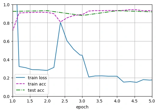
1 train_fine_tuning(finetune_net, 5e-5 )
1
2
3
4
5
epoch 1, loss 2.481, acc 0.708, test acc 0.924, time 22.67 sec epoch 2, loss 0.281, acc 0.912, test acc 0.931, time 19.62 sec epoch 3, loss 0.446, acc 0.888, test acc 0.879, time 19.63 sec epoch 4, loss 0.217, acc 0.932, test acc 0.931, time 19.73 sec epoch 5, loss 0.176, acc 0.930, test acc 0.919, time 19.72 sec
1
2
loss 0.176, train acc 0.930, test acc 0.919 339.0 examples/sec on [device(type='cuda', index=0)]
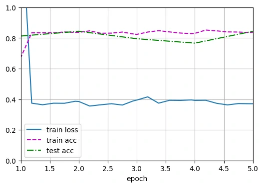
为了进行比较,定义了一个相同的模型,但是将其所有模型参数初始化为随机值,由于整个模型需要从头开始训练,因此需要使用更大的学习率
1
2
3
scratch_net = torchvision.models.resnet18() scratch_net.fc = nn.Linear(scratch_net.fc.in_features, 2 ) train_fine_tuning(scratch_net, 5e-4 , param_group=False )
1
2
3
4
5
epoch 1, loss 1.664, acc 0.673, test acc 0.812, time 19.94 sec epoch 2, loss 0.385, acc 0.837, test acc 0.844, time 19.95 sec epoch 3, loss 0.395, acc 0.824, test acc 0.795, time 19.47 sec epoch 4, loss 0.392, acc 0.830, test acc 0.766, time 19.94 sec epoch 5, loss 0.371, acc 0.836, test acc 0.844, time 19.73 sec
1
2
loss 0.371 , train acc 0.836 , test acc 0.844 340.4 examples/sec on [device(type ='cuda' , index=0 )]
意料之中,微调模型往往表现更好,因为它的初始参数值更有效
小结
迁移学习将从源数据集中学到的知识迁移到目标数据集,微调是迁移学习的常见技巧
除输出层外,目标模型从源模型中复制所有模型设计及其参数,并根据目标数据集对这些参数进行微调。但是目标模型的输出层需要从头开始训练
通常,微调参数使用较小的学习率,而从头开始训练输出层可以使用更大的学习率
思考题
将输出层finetune_net之前的参数设置为源模型的参数,在训练期间不要更新它们。模型的准确性如何变化?
1 2 3 4 5 6 7 for param in finetune_net.parameters(): param.requires_grad = False for param in finetune_net.fc.parameters(): param.requires_grad = True
冻结除输出层外的所有参数时模型训练更快、更稳定,但由于特征无法适应新任务,准确率通常比“微调全部层”略低
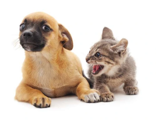
目标检测和边界框 在图像分类中通常假设图像只有一个主要目标,但若图像中存在多个对象,不仅要识别它们的类别,还要确定它们在图像中的位置,将这类任务称为目标检测(object detection)
目标检测在多个领域中被广泛使用,例如,在无人驾驶里,需要通过识别拍摄到的视频图像里的车辆、行人、道路和障碍物的位置来规划行进线路;机器人也常通过该任务来检测感兴趣的目标;安防领域则需要检测异常目标,如歹徒或者炸弹
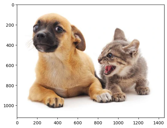
接下来以下图为例
1
2
3
4
img = Image.open ('imgs/catdog.jpg' ) plt.imshow(img) plt.axis('off' ) plt.show()
边界框 在目标检测中通常使用**边界框(bounding box)**来描述对象的空间位置
边界框是矩形的,由矩形左上角的以及右下角的$(x,y)$坐标决定,另一种常用的边界框表示方法是边界框中心的$(x,y)$坐标以及框的宽度和高度
定义在这两种表示法之间进行转换的函数
box_corner_to_center从两角表示法转换为中心宽度表示法,而box_center_to_corner反之
输入参数boxes可以是长度为4的张量,也可以是形状为$(n,4)$的二维张量,其中$n$是边界框的数量
1 2 3 4 5 6 7 8 9 10 11 12 13 14 15 16 17 18 19 20 21 22 23 def box_corner_to_center (boxes ): """从(左上,右下)转换到(中间,宽度,高度)""" x1, y1, x2, y2 = boxes[:, 0 ], boxes[:, 1 ], boxes[:, 2 ], boxes[:, 3 ] cx = (x1 + x2) / 2 cy = (y1 + y2) / 2 w = x2 - x1 h = y2 - y1 boxes = torch.stack((cx, cy, w, h), axis=-1 ) return boxes def box_center_to_corner (boxes ): """从(中间,宽度,高度)转换到(左上,右下)""" cx, cy, w, h = boxes[:, 0 ], boxes[:, 1 ], boxes[:, 2 ], boxes[:, 3 ] x1 = cx - 0.5 * w y1 = cy - 0.5 * h x2 = cx + 0.5 * w y2 = cy + 0.5 * h boxes = torch.stack((x1, y1, x2, y2), axis=-1 ) return boxes
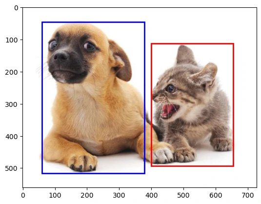
将根据坐标信息定义图像中狗和猫的边界框
图像中坐标的原点是图像的左上角,向右的方向为x轴的正方向,向下的方向为y轴的正方向
1 dog_bbox, cat_bbox = [60.0 , 45.0 , 378.0 , 516.0 ], [400.0 , 112.0 , 655.0 , 493.0 ]
通过转换两次来验证边界框转换函数的正确性
1
2
3
4
boxes = torch.tensor((dog_bbox, cat_bbox)) box_center_to_corner(box_corner_to_center(boxes)) == boxes
可以将边界框在图中画出,以检查其是否准确
画之前定义一个辅助函数bbox_to_rect,它将边界框表示成matplotlib的边界框格式
1 2 3 4 5 6 7 def bbox_to_rect (bbox, color ): return d2l.plt.Rectangle( xy=(bbox[0 ], bbox[1 ]), width=bbox[2 ]-bbox[0 ], height=bbox[3 ]-bbox[1 ], fill=False , edgecolor=color, linewidth=2 )
1
2
3
4
5
6
img = Image.open ('imgs/catdog.jpg' ) fig, ax = plt.subplots() ax.imshow(img) ax.add_patch(bbox_to_rect(dog_bbox, 'blue' )) ax.add_patch(bbox_to_rect(cat_bbox, 'red' )) plt.show()
锚框 目标检测算法通常会在输入图像中采样大量的区域然后判断这些区域中是否包含我们感兴趣的目标,并调整区域边界从而更准确地预测目标的真实边界框(ground-truth bounding box)
不同的模型使用的区域采样方法可能不同,这里使用的是以每个像素为中心,生成多个缩放比和宽高比(aspect ratio)不同的边界框,这些边界框被称为 锚框(anchor box)
修改输出精度,以获得更简洁的输出
1 torch.set_printoptions(2 )
生成多个锚框 假设输入图像的高度为$h$,高度为$w$,以图像的每个像素为中心生成不同形状的锚框:缩放比为$s\in (0, 1]$,宽高比为$r>0$
在实践中,只考虑包含$s_1$或$r_1$的组合
上述生成锚框的方法在下面的multibox_prior函数中实现,指定输入图像、尺寸列表和宽高比列表,然后此函数将返回所有的锚框
1 2 3 4 5 6 7 8 9 10 11 12 13 14 15 16 17 18 19 20 21 22 23 24 25 26 27 28 29 30 31 32 33 34 35 36 37 38 39 40 41 42 def multibox_prior (data, sizes, ratios ): """生成以每个像素为中心具有不同形状的锚框""" in_height, in_width = data.shape[-2 :] device, num_sizes, num_ratios = data.device, len (sizes), len (ratios) boxes_per_pixel = (num_sizes + num_ratios - 1 ) size_tensor = torch.tensor(sizes, device=device) ratio_tensor = torch.tensor(ratios, device=device) offset_h, offset_w = 0.5 , 0.5 steps_h = 1.0 / in_height steps_w = 1.0 / in_width center_h = (torch.arange(in_height, device=device) + offset_h) * steps_h center_w = (torch.arange(in_width, device=device) + offset_w) * steps_w shift_y, shift_x = torch.meshgrid(center_h, center_w, indexing='ij' ) shift_y, shift_x = shift_y.reshape(-1 ), shift_x.reshape(-1 ) w = (torch.cat((size_tensor * torch.sqrt(ratio_tensor[0 ]), sizes[0 ] * torch.sqrt(ratio_tensor[1 :]))) * in_height / in_width) h = torch.cat((size_tensor / torch.sqrt(ratio_tensor[0 ]), sizes[0 ] / torch.sqrt(ratio_tensor[1 :]))) anchor_manipulations = torch.stack((-w, -h, w, h)).T.repeat(in_height * in_width, 1 ) / 2 out_grid = torch.stack([shift_x, shift_y, shift_x, shift_y], dim=1 ).repeat_interleave(boxes_per_pixel, dim=0 ) output = out_grid + anchor_manipulations return output.unsqueeze(0 )
返回的锚框变量Y的形状是(批量大小,锚框的数量,4)
1
2
3
4
5
img = Image.open ('imgs/catdog.jpg' ) w, h = img.size X = torch.rand(size=(1 , 3 , h, w)) Y = multibox_prior(X, sizes=[0.75 , 0.5 , 0.25 ], ratios=[1 , 2 , 0.5 ]) boxes = Y.reshape(h, w, 5 , 4 )
将锚框变量Y的形状更改为(图像高度,图像宽度,以同一像素为中心的锚框的数量,4)后可以获得以指定像素的位置为中心的所有锚框
1 boxes = Y.reshape(h, w, 5 , 4 )
访问以(250,250)为中心的第一个锚框
1 tensor([0.06, 0.07, 0.63, 0.82])
为了显示以图像中以某个像素为中心的所有锚框,定义下面的show_bboxes函数来在图像上绘制多个边界框
1 2 3 4 5 6 7 8 9 10 11 12 13 14 15 16 17 18 19 20 21 22 23 24 25 26 27 28 29 30 def show_bboxes (axes, bboxes, labels=None , colors=None ): """显示所有边界框""" def _make_list (obj, default_values=None ): if obj is None : obj = default_values elif not isinstance (obj, (list , tuple )): obj = [obj] return obj labels = _make_list(labels) colors = _make_list(colors, ['b' , 'g' , 'r' , 'm' , 'c' ]) for i, bbox in enumerate (bboxes): color = colors[i % len (colors)] rect = bbox_to_rect(bbox.detach().numpy(), color) axes.add_patch(rect) if labels and len (labels) > i: text_color = 'k' if color == 'w' else 'w' axes.text(rect.xy[0 ], rect.xy[1 ], labels[i], va='center' , ha='center' , fontsize=9 , color=text_color, bbox=dict (facecolor=color, lw=0 ))
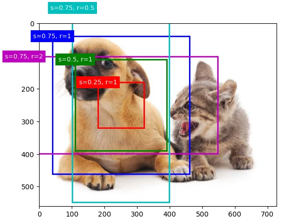
变量boxes中xy轴的坐标值已经分别除以图像的宽度和高度,绘制锚框时需要恢复它们原始的坐标值,在下面定义了变量bbox_scale,现在可以绘制出图像中所有以(250,250)为中心的锚框了
1
2
3
4
5
6
bbox_scale = torch.tensor((w, h, w, h)) fig, ax = plt.subplots() ax.imshow(img) show_bboxes(ax, boxes[250 , 250 , :, :] * bbox_scale, ['s=0.75, r=1' , 's=0.5, r=1' , 's=0.25, r=1' , 's=0.75, r=2' , 's=0.75, r=0.5' ])
缩放比为0.75且宽高比为1的蓝色锚框很好地围绕着图像中的狗
交并比(IoU) 如果已知目标的真实边界框,那么这里的“好”该如何如何量化呢?
直观地说,可以衡量锚框和真实边界框之间的相似性
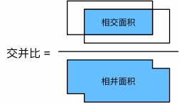
杰卡德系数(Jaccard)可以衡量两组之间的相似性,给定集合$\mathcal{A}$和$\mathcal{B}$,他们的杰卡德系数是他们交集的大小除以他们并集的大小: (intersection over union,IoU) ,即两个边界框相交面积与相并面积之比
交并比的取值范围在0和1之间:0表示两个边界框无重合像素,1表示两个边界框完全重合
接下来部分将使用交并比来衡量锚框和真实边界框之间、以及不同锚框之间的相似度
给定两个锚框或边界框的列表,以下box_iou函数将在这两个列表中计算它们成对的交并比
1 2 3 4 5 6 7 8 9 10 11 12 13 14 15 16 17 18 19 20 def box_iou (boxes1, boxes2 ): """计算两个锚框或边界框列表中成对的交并比""" box_area = lambda boxes: ((boxes[:, 2 ] - boxes[:, 0 ]) * (boxes[:, 3 ] - boxes[:, 1 ])) areas1 = box_area(boxes1) areas2 = box_area(boxes2) inter_upperlefts = torch.max (boxes1[:, None , :2 ], boxes2[:, :2 ]) inter_lowerrights = torch.min (boxes1[:, None , 2 :], boxes2[:, 2 :]) inters = (inter_lowerrights - inter_upperlefts).clamp(min =0 ) inter_areas = inters[:, :, 0 ] * inters[:, :, 1 ] union_areas = areas1[:, None ] + areas2 - inter_areas return inter_areas / union_areas
在训练数据中标注锚框 在目标检测中,每个锚框都作为一个训练样本,需要预测类别和位置偏移。训练时将锚框与最接近的真实边界框匹配,赋予对应的类别和偏移标签;预测时生成所有锚框的类别与偏移,并根据偏移调整锚框位置,最后筛选出符合条件的预测框
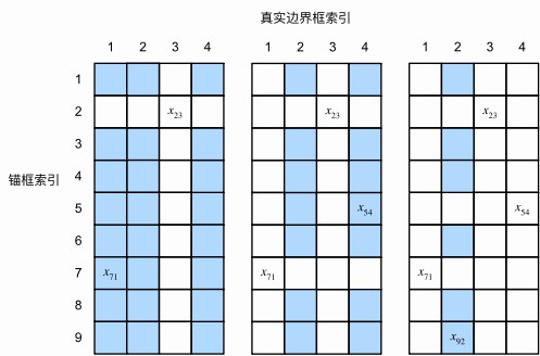
将真实边界框分配给锚框 给定图像,假设锚框是$A_1, A_2, \ldots, A_{n_a}$,真实边界框是$B_1, B_2, \ldots, B_{n_b}$,其中$n_a \geq n_b$,定义一个矩阵$\mathbf X \in \mathbb{R}^{n_a \times n_b}$,其中第$i$行第$j$列的元素$x_{ij}$是锚框$A_i$和真实边界框$B_j$的IoU,该算法包含以下步骤
在IoU矩阵中找到最大的元素,其行列索引分别对应一个锚框和真实边界框,将该真实边界框分配给该锚框,并从IoU矩阵中删除对应的行和列
重复上述步骤,直到每个真实边界框都分配给一个锚框为止
对剩余未分配的$n_a-n_b$个锚框,找到 IoU 最大的真实边界框;若该 IoU 大于预设阈值,则将该真实框分配给该锚框
用一个具体的例子来说明上述算法
假设矩阵中的最大值为$x_{23}$,将真实边界框$B_3$分配给$A_2$,然后丢弃矩阵第2行和第3列中的所有元素(左图);在剩余元素(阴影区域)中找到最大的$x_{71}$,然后将真实边界框$B_1$分配给$A_7$,丢弃矩阵第7行和第1列中的所有元素(中图);在剩余元素(阴影区域)中找到最大的$x_{54}$,然后将真实边界框$B_4$分配给锚框$A_5$,丢弃后在剩余找到最大的$x_{92}$,然后将真实边界框$B_2$分配给锚框$A_9$(右图);最后遍历剩余的锚框$A_1, A_3, A_4, A_6, A_8$,然后根据阈值判断是否为它们分配真实边界框
此算法在下面的assign_anchor_to_bbox函数中实现
1 2 3 4 5 6 7 8 9 10 11 12 13 14 15 16 17 18 19 20 21 22 23 24 25 26 27 28 29 30 31 32 33 34 35 36 37 38 39 40 41 42 def assign_anchor_to_bbox (ground_truth, anchors, device, iou_threshold=0.5 ): """ 将每个锚框(anchor)分配给最接近的真实边界框(ground truth box)。 参数: ground_truth : (n_gt, 4) anchors : (n_anchor, 4) iou_threshold : 超过该值的锚框才会被视为“正样本”(即分配给某个真实框) 返回: anchors_bbox_map : (n_anchor,) 其中第 i 个元素表示该锚框对应的真实边界框索引; 若值为 -1,表示该锚框未分配(负样本) """ num_anchors, num_gt_boxes = anchors.shape[0 ], ground_truth.shape[0 ] jaccard = box_iou(anchors, ground_truth) anchors_bbox_map = torch.full((num_anchors,), -1 , dtype=torch.long, device=device) max_ious, indices = torch.max (jaccard, dim=1 ) anc_i = torch.nonzero(max_ious >= iou_threshold).reshape(-1 ) box_j = indices[max_ious >= iou_threshold] anchors_bbox_map[anc_i] = box_j col_discard = torch.full((num_anchors,), -1 ) row_discard = torch.full((num_gt_boxes,), -1 ) for _ in range (num_gt_boxes): max_idx = torch.argmax(jaccard) box_idx = (max_idx % num_gt_boxes).long() anc_idx = (max_idx / num_gt_boxes).long() anchors_bbox_map[anc_idx] = box_idx jaccard[:, box_idx] = col_discard jaccard[anc_idx, :] = row_discard return anchors_bbox_map
标记类别和偏移量 现在可以为每个锚框标记类别和偏移量了,假设一个锚框$A$被分配给了一个真实边界框$B$
一方面,锚框A的类别将被标记为与B相同,另一方面,锚框A的偏移量将根据B和A中心坐标的相对位置以及这两个框的相对大小进行标记,鉴于数据集内不同的框的位置和大小不同,可以对那些相对位置和大小应用变换,使其获得分布更均匀且易于拟合的偏移量
可以将A的偏移量标记为:offset_boxes函数中实现
1 2 3 4 5 6 7 8 9 10 11 12 def offset_boxes (anchors, assigned_bb, eps=1e-6 ): """对锚框偏移量的转换""" c_anc = box_corner_to_center(anchors) c_assigned_bb = box_corner_to_center(assigned_bb) offset_xy = 10 * (c_assigned_bb[:, :2 ] - c_anc[:, :2 ]) / c_anc[:, 2 :] offset_wh = 5 * torch.log(eps + c_assigned_bb[:, 2 :] / c_anc[:, 2 :]) offset = torch.cat([offset_xy, offset_wh], axis=1 ) return offset
如果一个锚框没有被分配真实边界框,只需将锚框的类别标记为背景(background),背景类别的锚框通常被称为负类锚框,其余的被称为正类锚框
使用真实边界框(labels参数)实现以下multibox_target函数,来标记锚框的类别和偏移量(anchors参数)
此函数将背景类别的索引设置为零,然后将新类别的整数索引递增一
1 2 3 4 5 6 7 8 9 10 11 12 13 14 15 16 17 18 19 20 21 22 23 24 25 26 27 28 29 30 31 32 33 34 35 36 37 38 39 40 41 42 43 44 45 46 47 48 49 50 51 52 def multibox_target (anchors, labels ): """使用真实边界框标记锚框 参数 anchors : torch.Tensor, 形状 (1, num_anchors, 4) 所有锚框的坐标 [xmin, ymin, xmax, ymax],通常来自 multibox_prior() labels : torch.Tensor, 形状 (batch_size, num_objects, 5) 每张图片的真实标注,格式为 [class, xmin, ymin, xmax, ymax] - class = 目标类别编号(从0开始) - 没有目标的地方通常用0填充 返回 bbox_offset : torch.Tensor, 形状 (batch_size, num_anchors * 4) 每个锚框相对于匹配的真实框的偏移量(训练回归目标) bbox_mask : torch.Tensor, 形状 (batch_size, num_anchors * 4) 掩码,标记哪些锚框是真实匹配(1)哪些是背景(0) class_labels : torch.Tensor, 形状 (batch_size, num_anchors) 每个锚框的类别标签(0 表示背景) """ batch_size, anchors = labels.shape[0 ], anchors.squeeze(0 ) batch_offset, batch_mask, batch_class_labels = [], [], [] device, num_anchors = anchors.device, anchors.shape[0 ] for i in range (batch_size): label = labels[i, :, :] anchors_bbox_map = assign_anchor_to_bbox( label[:, 1 :], anchors, device) bbox_mask = ((anchors_bbox_map >= 0 ).float ().unsqueeze(-1 )).repeat( 1 , 4 ) class_labels = torch.zeros(num_anchors, dtype=torch.long, device=device) assigned_bb = torch.zeros((num_anchors, 4 ), dtype=torch.float32, device=device) indices_true = torch.nonzero(anchors_bbox_map >= 0 ) bb_idx = anchors_bbox_map[indices_true] class_labels[indices_true] = label[bb_idx, 0 ].long() + 1 assigned_bb[indices_true] = label[bb_idx, 1 :] offset = offset_boxes(anchors, assigned_bb) * bbox_mask batch_offset.append(offset.reshape(-1 )) batch_mask.append(bbox_mask.reshape(-1 )) batch_class_labels.append(class_labels) bbox_offset = torch.stack(batch_offset) bbox_mask = torch.stack(batch_mask) class_labels = torch.stack(batch_class_labels) return (bbox_offset, bbox_mask, class_labels)
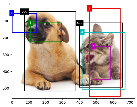
例子 通过一个具体的例子来说明锚框标签,已经为加载图像中的狗和猫定义了真实边界框,其中第一个元素是类别(0代表狗,1代表猫),其余四个元素是左上角和右下角的轴坐标(范围介于0和1之间)
还构建了五个锚框,用左上角和右下角的坐标进行标记$A_0, \ldots, A_4$(索引从0开始),然后在图像中绘制这些真实边界框和锚框
1
2
3
4
5
6
7
8
9
10
ground_truth = torch.tensor([[0 , 0.1 , 0.08 , 0.52 , 0.92 ], [1 , 0.55 , 0.2 , 0.9 , 0.88 ]]) anchors = torch.tensor([[0 , 0.1 , 0.2 , 0.3 ], [0.15 , 0.2 , 0.4 , 0.4 ], [0.63 , 0.05 , 0.88 , 0.98 ], [0.66 , 0.45 , 0.8 , 0.8 ], [0.57 , 0.3 , 0.92 , 0.9 ]]) img = Image.open ('imgs/catdog.jpg' ) fig, ax = plt.subplots() ax.imshow(img) show_bboxes(ax, ground_truth[:, 1 :] * bbox_scale, ['dog' , 'cat' ], 'k' ) show_bboxes(ax, anchors * bbox_scale, ['0' , '1' , '2' , '3' , '4' ]);
使用上面定义的multibox_target函数,可以根据狗和猫的真实边界框,标注这些锚框的分类和偏移量
为锚框和真实边界框样本添加一个维度
1
2
3
labels = multibox_target(anchors.unsqueeze(dim=0 ), ground_truth.unsqueeze(dim=0 )) labels[2 ]
返回的结果中有三个元素,都是张量格式,第三个元素包含标记的输入锚框的类别
1 tensor([[0, 1, 2, 0, 2]])
返回的第二个元素是掩码(mask)变量,形状为(批量大小,锚框数的四倍)
掩码变量中的元素与每个锚框的4个偏移量一一对应
由于不关心对背景的检测,负类的偏移量不应影响目标函数,通过元素乘法,掩码变量中的零将在计算目标函数之前过滤掉负类偏移量
使用非极大值抑制预测边界框 在预测时,先为图像生成多个锚框,再为这些锚框一一预测类别和偏移量,一个预测好的边界框则根据其中某个带有预测偏移量的锚框而生成
实现的offset_inverse函数,该函数将锚框和偏移量预测作为输入,并应用逆偏移变换来返回预测的边界框坐标
当有许多锚框时,可能会输出许多相似的具有明显重叠的预测边界框,都围绕着同一目标,为了简化输出,可以使用**非极大值抑制(non-maximum suppression,NMS)**合并属于同一目标的类似的预测边界框
目标检测模型会计算每个类别的预测概率,在同一张图像中,所有预测的非背景边界框都按置信度降序排序,以生成列表$L$
选出置信度最高的预测框作为基准
删除所有与该框的 IoU 大于阈值的其他预测框
对剩余框重复以上步骤,直到没有可删除的框为止
输出保留的预测框集合
以下nms函数按降序对置信度进行排序并返回其索引
1 2 3 4 5 6 7 8 9 10 11 12 13 14 def nms (boxes, scores, iou_threshold ): """对预测边界框的置信度进行排序""" B = torch.argsort(scores, dim=-1 , descending=True ) keep = [] while B.numel() > 0 : i = B[0 ] keep.append(i) if B.numel() == 1 : break iou = box_iou(boxes[i, :].reshape(-1 , 4 ), boxes[B[1 :], :].reshape(-1 , 4 )).reshape(-1 ) inds = torch.nonzero(iou <= iou_threshold).reshape(-1 ) B = B[inds + 1 ] return torch.tensor(keep, device=boxes.device)
定义以下multibox_detection函数来将非极大值抑制应用于预测边界框
1 2 3 4 5 6 7 8 9 10 11 12 13 14 15 16 17 18 19 20 21 22 23 24 25 26 27 28 29 30 31 32 def multibox_detection (cls_probs, offset_preds, anchors, nms_threshold=0.5 , pos_threshold=0.009999999 ): """使用非极大值抑制来预测边界框""" device, batch_size = cls_probs.device, cls_probs.shape[0 ] anchors = anchors.squeeze(0 ) num_classes, num_anchors = cls_probs.shape[1 ], cls_probs.shape[2 ] out = [] for i in range (batch_size): cls_prob, offset_pred = cls_probs[i], offset_preds[i].reshape(-1 , 4 ) conf, class_id = torch.max (cls_prob[1 :], 0 ) predicted_bb = offset_inverse(anchors, offset_pred) keep = nms(predicted_bb, conf, nms_threshold) all_idx = torch.arange(num_anchors, dtype=torch.long, device=device) combined = torch.cat((keep, all_idx)) uniques, counts = combined.unique(return_counts=True ) non_keep = uniques[counts == 1 ] all_id_sorted = torch.cat((keep, non_keep)) class_id[non_keep] = -1 class_id = class_id[all_id_sorted] conf, predicted_bb = conf[all_id_sorted], predicted_bb[all_id_sorted] below_min_idx = (conf < pos_threshold) class_id[below_min_idx] = -1 conf[below_min_idx] = 1 - conf[below_min_idx] pred_info = torch.cat((class_id.unsqueeze(1 ), conf.unsqueeze(1 ), predicted_bb), dim=1 ) out.append(pred_info) return torch.stack(out)
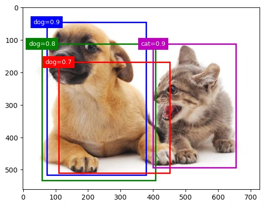
现在将上述算法应用到一个带有四个锚框的具体示例中,为简单起见,假设预测的偏移量都是零,这意味着预测的边界框即是锚框。 对于背景、狗和猫其中的每个类,还定义了它的预测概率
1
2
3
4
5
6
anchors = torch.tensor([[0.1 , 0.08 , 0.52 , 0.92 ], [0.08 , 0.2 , 0.56 , 0.95 ], [0.15 , 0.3 , 0.62 , 0.91 ], [0.55 , 0.2 , 0.9 , 0.88 ]]) offset_preds = torch.tensor([0 ] * anchors.numel()) cls_probs = torch.tensor([[0 ] * 4 , [0.9 , 0.8 , 0.7 , 0.1 ], [0.1 , 0.2 , 0.3 , 0.9 ]])
在图像上绘制这些预测边界框和置信度
可以调用multibox_detection函数来执行非极大值抑制,其中阈值设置为0.5
可以看到返回结果的形状是(批量大小,锚框的数量,6),最内层维度中的六个元素提供了同一预测边界框的输出信息
第一个元素是预测的类索引,从0开始(0代表狗,1代表猫),值-1表示背景或在非极大值抑制中被移除了,第二个元素是预测的边界框的置信度,其余四个元素是坐标
1
2
3
4
5
output = multibox_detection(cls_probs.unsqueeze(dim=0 ), offset_preds.unsqueeze(dim=0 ), anchors.unsqueeze(dim=0 ), nms_threshold=0.5 ) output
1
2
3
4
tensor([[[ 0.00, 0.90, 0.10, 0.08, 0.52, 0.92], [ 1.00, 0.90, 0.55, 0.20, 0.90, 0.88], [-1.00, 0.80, 0.08, 0.20, 0.56, 0.95], [-1.00, 0.70, 0.15, 0.30, 0.62, 0.91]]])
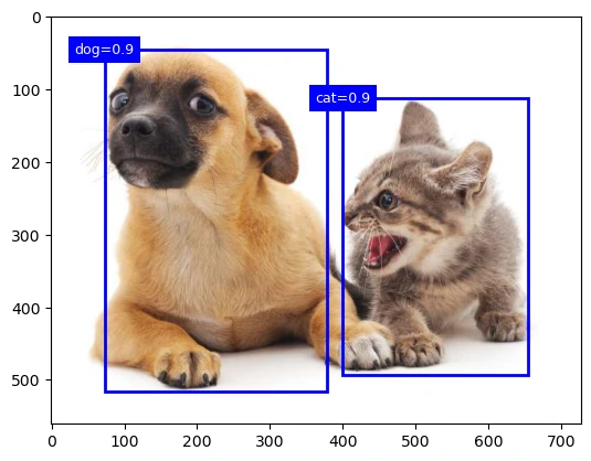
删除-1类别(背景)的预测边界框后,可以输出由非极大值抑制保存的最终预测边界框
1
2
3
4
5
6
7
_, ax = plt.subplots() ax.imshow(img) for i in output[0 ].detach().numpy(): if i[0 ] == -1 : continue label = ('dog=' , 'cat=' )[int (i[0 ])] + str (i[1 ]) show_bboxes(ax, [torch.tensor(i[2 :]) * bbox_scale], label)
区域卷积神经网络(R-CNN) 区域卷积神经网络(region-based CNN或regions with CNN features,R-CNN)(Girshick et al. , 2014)也是将深度模型应用于目标检测的开创性工作之一
本节将介绍R-CNN及其一系列改进方法:快速的R-CNN(Fast R-CNN)(Girshick, 2015)、更快的R-CNN(Faster R-CNN) (Ren et al. , 2015 )和掩码R-CNN(Mask R-CNN)(He et al. , 2017)
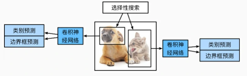
R-CNN R-CNN首先从输入图像中选取若干(例如2000个)提议区域(如锚框也是一种选取方法),并标注它们的类别和边界框(如偏移量),用卷积神经网络对每个提议区域进行前向传播以抽取其特征,用每个提议区域的特征来预测类别和边界框
R-CNN包括以下四个步骤:
对输入图像使用选择性搜索来选取多个高质量的提议区域(Uijlings et al. , 2013),这些区域覆盖不同尺度、形状和位置。每个候选区域都会被标注所属类别及对应的真实边界框
选择一个预训练的卷积神经网络,截取到输出层之前的部分,将每个提议区域裁剪并缩放到网络输入尺寸,通过前向传播得到其特征向量
把每个区域的特征与标签作为样本,训练多个支持向量机(SVM),每个 SVM 负责判断该区域是否属于特定类别
将每个提议区域的特征连同其标注的边界框作为一个样本,训练线性回归模型来预测真实边界框
尽管R-CNN模型通过预训练的卷积神经网络有效地抽取了图像特征,但它的速度很慢,可能从一张图像中选出上千个提议区域,这需要上千次的卷积神经网络的前向传播来执行目标检测,这种庞大的计算量使得R-CNN在现实世界中难以被广泛应用
Fast R-CNN R-CNN的主要性能瓶颈在于,对每个提议区域,卷积神经网络的前向传播是独立的,而没有共享计算
由于这些区域通常有重叠,独立的特征抽取会导致重复的计算,Fast R-CNN(Girshick, 2015)对R-CNN的主要改进之一,是仅在整张图象上执行卷积神经网络的前向传播
它的主要计算如下:
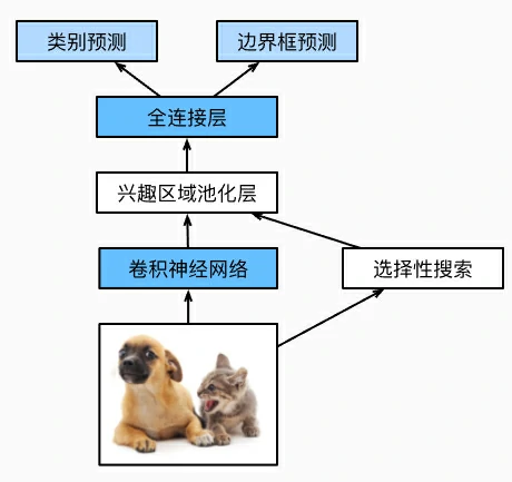
与 R-CNN 逐个裁剪区域再提特征不同,Fast R-CNN直接把整张图像输入卷积神经网络。网络输出一个特征图,形状为$1 \times c \times h_1 \times w_1$,这一步只需一次前向传播即可完成所有区域的特征提取
选择性搜索生成 $n$ 个提议区域(RoI),每个区域在特征图上被定位后,通过**兴趣区域汇聚层(RoI Pooling)**变换为固定大小(例如$h_2\times w_2$)的特征块,每个 RoI 都会输出统一形状的特征张量$n \times c \times h_2 \times w_2$
将每个 RoI 的特征展平并输入全连接层,得到$n \times d$的向量表示,其中超参数$d$取决于模型设计
网络分为两个并行的分支,类别预测输出每个 RoI 属于各类别的概率分布,形状为$n \times q$并使用 softmax;边界框预测输出每个 RoI 的边界框偏移量,形状为$n \times 4$
在Fast R-CNN中提出的RoI Pooling与之前介绍的汇聚层有所不同,汇聚层的输出形状是通过卷积核大小、填充方式和步幅 间接决定的,而RoI Pooling可以直接指定每个兴趣区域的输出尺寸
对于任何形状为$h \times w$的兴趣区域窗口,该窗口将被划分为$h_2 \times w_2$子窗口网格,其中每个子窗口的大小约为$(h/h_2) \times (w/w_2)$,在实际计算中,这些子窗口的宽高都会向上取整,以确保覆盖完整区域,取其中的最大元素作为该子窗口的输出
这样兴趣区域汇聚层可从形状各异的兴趣区域中均抽取出形状相同的特征
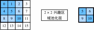
下面演示兴趣区域汇聚层的计算方法,假设卷积神经网络抽取的特征X的高度和宽度都是4,且只有单通道
假设输入图像的高度和宽度都是40,且选择性搜索在此图像上生成了两个提议区域,每个区域由5个元素表示:区域目标类别、左上角和右下角的坐标
1
2
X = torch.arange(16 , dtype=torch.float32).reshape(1 ,1 ,4 ,4 ) rois = torch.Tensor([[0 , 0 , 0 , 20 , 20 ], [0 , 0 , 10 , 30 , 30 ]])
由于X的高和宽是输入图像高和宽的$1/10$,两个提议区域的坐标先按spatial_scale乘以0.1,然后在X上分别标出这两个兴趣区域X[:, :, 0:3, 0:3] X[:, :, 1:4, 0:4]
在2×2的兴趣区域汇聚层中,每个兴趣区域被划分为子窗口网格,并进一步抽取相同形状的特征
1 torchvision.ops.roi_pool(X, rois, output_size=(2 , 2 ), spatial_scale=0.1 )
1
2
3
4
5
6
tensor([[[[ 5., 6.], [ 9., 10.]]], [[[ 9., 11.], [13., 15.]]]])
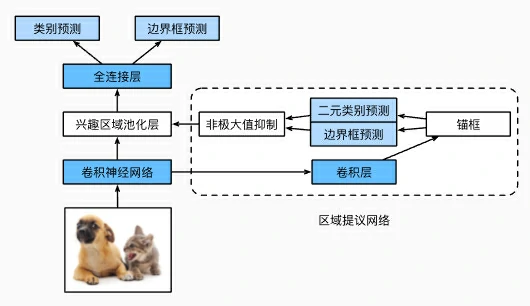
Faster R-CNN 为了较精确地检测目标结果,Fast R-CNN模型通常需要在选择性搜索中生成大量的提议区域
Faster R-CNN (Ren et al. , 2015)提出将选择性搜索替换为区域提议网络(region proposal network) ,从而减少提议区域的生成数量,并保证目标检测的精度
与Fast R-CNN相比,Faster R-CNN只将生成提议区域的方法从选择性搜索改为了区域提议网络,模型的其余部分保持不变
区域提议网络的计算步骤如下:
使用填充为1的3×3卷积层变换卷积神经网络的输出,输出通道为$c$,把每个特征图位置的上下文揉成一条长度为$c$的新特征
以特征图的每个像素为中心,生成多个不同大小和宽高比的锚框并标注它们
使用锚框中心单元长度为$c$的特征,分别预测该锚框的二元类别(含目标还是背景)和边界框
使用非极大值抑制,从预测类别为目标的预测边界框中移除相似的结果,最终输出的预测边界框即是兴趣区域汇聚层所需的提议区域
区域提议网络作为Faster R-CNN模型的一部分,是和整个模型一起训练得到的
Faster R-CNN的目标函数不仅包括目标检测中的类别和边界框预测,还包括区域提议网络中锚框的二元类别和边界框预测
作为端到端训练的结果,区域提议网络能够学习到如何生成高质量的提议区域,从而在减少了从数据中学习的提议区域的数量的情况下,仍保持目标检测的精度
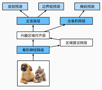
Mask R-CNN 如果在训练集中还标注了每个目标在图像上的像素级位置,那么Mask R-CNN(He et al. , 2017)能够有效地利用这些详尽的标注信息进一步提升目标检测的精度
Mask R-CNN是基于Faster R-CNN修改而来的
Mask R-CNN将兴趣区域汇聚层替换为了兴趣区域对齐层 ,使用**双线性插值(bilinear interpolation)**来保留特征图上的空间信息,从而更适于像素级预测
兴趣区域对齐层的输出包含了所有与兴趣区域的形状相同的特征图,不仅被用于预测每个兴趣区域的类别和边界框,还通过额外的全卷积网络预测目标的像素级位置
小结
R-CNN对图像选取若干提议区域,使用卷积神经网络对每个提议区域执行前向传播以抽取其特征,然后再用这些特征来预测提议区域的类别和边界框
Fast R-CNN对R-CNN的一个主要改进:只对整个图像做卷积神经网络的前向传播,它还引入了兴趣区域汇聚层,从而为具有不同形状的兴趣区域抽取相同形状的特征
Faster R-CNN将Fast R-CNN中使用的选择性搜索替换为参与训练的区域提议网络,这样后者可以在减少提议区域数量的情况下仍保证目标检测的精度
Mask R-CNN在Faster R-CNN的基础上引入了一个全卷积网络,从而借助目标的像素级位置进一步提升目标检测的精度
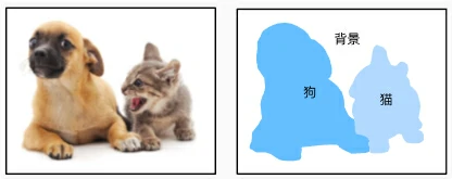
语义分割和数据集 之前一直使用方形边界框来标注和预测图像中的目标,**语义分割(semantic segmentation)**重点关注于如何将图像分割成属于不同语义类别的区域
与目标检测不同,语义分割可以识别并理解图像中每一个像素的内容,标注和预测是像素级的,语义分割标注的像素级的边框显然更加精细
图像分割和实例分割 计算机视觉领域还有2个与语义分割相似的重要问题,即图像分割(image segmentation)和 实例分割(instance segmentation)
图像分割将图像划分为若干组成区域,这类问题的方法通常利用图像中像素之间的相关性,它在训练时不需要有关图像像素的标签信息,在预测时也无法保证分割出的区域具有我们希望得到的语义;图像分割可能会将狗分为两个区域:一个覆盖以黑色为主的嘴和眼睛,另一个覆盖以黄色为主的其余部分身体
实例分割也叫同时检测并分割(simultaneous detection and segmentation) ,它研究如何识别图像中各个目标实例的像素级区域,与语义分割不同,实例分割不仅需要区分语义,还要区分不同的目标实例;如果图像中有两条狗,则实例分割需要区分像素属于的两条狗中的哪一条
Pascal VOC2012 最重要的语义分割数据集之一是Pascal VOC2012
数据集的tar文件大约为2GB,所以下载可能需要一段时间,提取出的数据集位于../data/VOCdevkit/VOC2012
1 2 3 4 DATA_HUB['voc2012' ] = ( DATA_URL + 'VOCtrainval_11-May-2012.tar' , '4e443f8a2eca6b1dac8a6c57641b67dd40621a49' ) voc_dir = download_extract('voc2012' , 'VOCdevkit/VOC2012' )
1 voc_dir = download_extract('voc2012' , 'VOCdevkit/VOC2012' )
进入路径../data/VOCdevkit/VOC2012之后可以看到数据集的不同组件
ImageSets/Segmentation路径包含用于训练和测试样本的文本文件,而JPEGImages和SegmentationClass路径分别存储着每个示例的输入图像和标签
1 2 3 4 5 6 7 8 9 10 11 12 13 14 15 16 17 def read_voc_images (voc_dir, is_train=True ): """读取所有VOC图像并标注""" txt_fname = os.path.join(voc_dir, 'ImageSets' , 'Segmentation' , 'train.txt' if is_train else 'val.txt' ) mode = torchvision.io.image.ImageReadMode.RGB with open (txt_fname, 'r' ) as f: images = f.read().split() features, labels = [], [] for i, fname in enumerate (images): features.append(torchvision.io.read_image(os.path.join( voc_dir, 'JPEGImages' , f'{fname} .jpg' ))) labels.append(torchvision.io.read_image(os.path.join( voc_dir, 'SegmentationClass' ,f'{fname} .png' ), mode)) return features, labels
1 train_features, train_labels = read_voc_images(voc_dir, True )
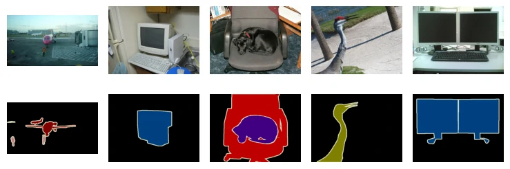
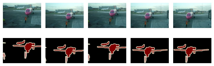
绘制前5个输入图像及其标签,在标签图像中,白色和黑色分别表示边框和背景,而其他颜色则对应不同的类别
1
2
3
4
5
6
n = 5 imgs = train_features[0 :n] + train_labels[0 :n] imgs = [img.permute(1 ,2 ,0 ) for img in imgs] show_images(imgs, 2 , n);
列举RGB颜色值和类名
1 2 3 4 5 6 7 8 9 10 11 12 13 VOC_COLORMAP = [[0 , 0 , 0 ], [128 , 0 , 0 ], [0 , 128 , 0 ], [128 , 128 , 0 ], [0 , 0 , 128 ], [128 , 0 , 128 ], [0 , 128 , 128 ], [128 , 128 , 128 ], [64 , 0 , 0 ], [192 , 0 , 0 ], [64 , 128 , 0 ], [192 , 128 , 0 ], [64 , 0 , 128 ], [192 , 0 , 128 ], [64 , 128 , 128 ], [192 , 128 , 128 ], [0 , 64 , 0 ], [128 , 64 , 0 ], [0 , 192 , 0 ], [128 , 192 , 0 ], [0 , 64 , 128 ]] VOC_CLASSES = ['background' , 'aeroplane' , 'bicycle' , 'bird' , 'boat' , 'bottle' , 'bus' , 'car' , 'cat' , 'chair' , 'cow' , 'diningtable' , 'dog' , 'horse' , 'motorbike' , 'person' , 'potted plant' , 'sheep' , 'sofa' , 'train' , 'tv/monitor' ]
通过上面定义的两个常量,可以方便地查找标签中每个像素的类索引
定义voc_colormap2label函数来构建从上述RGB颜色值到类别索引的映射,而voc_label_indices函数将RGB值映射到在Pascal VOC2012数据集中的类别索引
1 2 3 4 5 6 7 8 9 10 11 12 13 14 15 def voc_colormap2label (): """构建从RGB到VOC类别索引的映射""" colormap2label = torch.zeros(256 ** 3 , dtype=torch.long) for i, colormap in enumerate (VOC_COLORMAP): colormap2label[ (colormap[0 ] * 256 + colormap[1 ]) * 256 + colormap[2 ]] = i return colormap2label def voc_label_indices (colormap, colormap2label ): """将VOC标签中的RGB值映射到它们的类别索引""" colormap = colormap.permute(1 , 2 , 0 ).numpy().astype('int32' ) idx = ((colormap[:, :, 0 ] * 256 + colormap[:, :, 1 ]) * 256 + colormap[:, :, 2 ]) return colormap2label[idx]
例如,在第一张样本图像中,飞机头部区域的类别索引为1,而背景索引为0
1
2
y = voc_label_indices(train_labels[0 ], voc_colormap2label()) y[105 :115 , 130 :140 ], VOC_CLASSES[1 ]
1
2
3
4
5
6
7
8
9
10
11
(tensor([[0, 0, 0, 0, 0, 0, 0, 0, 0, 1], [0, 0, 0, 0, 0, 0, 0, 1, 1, 1], [0, 0, 0, 0, 0, 0, 1, 1, 1, 1], [0, 0, 0, 0, 0, 1, 1, 1, 1, 1], [0, 0, 0, 0, 0, 1, 1, 1, 1, 1], [0, 0, 0, 0, 1, 1, 1, 1, 1, 1], [0, 0, 0, 0, 0, 1, 1, 1, 1, 1], [0, 0, 0, 0, 0, 1, 1, 1, 1, 1], [0, 0, 0, 0, 0, 0, 1, 1, 1, 1], [0, 0, 0, 0, 0, 0, 0, 0, 1, 1]]), 'aeroplane')
预处理数据 在之前的实验通过再缩放图像使其符合模型的输入形状,在语义分割中,这样做需要将预测的像素类别重新映射回原始尺寸的输入图像,这样的映射可能不够精确,尤其在不同语义的分割区域
为了避免这个问题,将图像裁剪为固定尺寸,而不是再缩放,使用图像增广中的随机裁剪,裁剪输入图像和标签的相同区域
1
2
3
4
5
6
7
def voc_rand_crop (feature,label,height, width ): """随机裁剪特征和标签图像""" rect = torchvision.transforms.RandomCrop.get_params( feature, (height, width)) feature = torchvision.transforms.functional.crop(feature, *rect) label = torchvision.transforms.functional.crop(label, *rect) return feature, label
1
2
3
4
5
6
imgs = [] for _ in range (n): imgs += voc_rand_crop(train_features[0 ], train_labels[0 ], 200 , 300 ) imgs = [img.permute(1 , 2 , 0 ) for img in imgs] show_images(imgs[::2 ] + imgs[1 ::2 ], 2 , n);
自定义语义分割数据集类 通过继承高级API提供的Dataset类,自定义了一个语义分割数据集类VOCSegDataset
通过实现__getitem__函数,可以任意访问数据集中索引为idx的输入图像及其每个像素的类别索引
由于数据集中有些图像的尺寸可能小于随机裁剪所指定的输出尺寸,这些样本可以通过自定义的filter函数移除掉
还定义了normalize_image函数,从而对输入图像的RGB三个通道的值分别做标准化
1
2
3
4
5
6
7
8
9
10
11
12
13
14
15
16
17
18
19
20
21
22
23
24
25
26
27
28
29
class VOCSegDataset (torch.utils.data.Dataset): """一个用于加载VOC数据集的自定义数据集""" def __init__ (self, is_train, crop_size, voc_dir ): self .transform = torchvision.transforms.Normalize( mean=[0.485 , 0.456 , 0.406 ], std=[0.229 , 0.224 , 0.225 ]) self .crop_size = crop_size features, labels = read_voc_images(voc_dir, is_train=is_train) self .features = [self .normalize_image(feature) for feature in self .filter (features)] self .labels = self .filter (labels) self .colormap2label = voc_colormap2label() print ('read ' + str (len (self .features)) + ' examples' ) def normalize_image (self, img ): return self .transform(img.float () / 255 ) def filter (self, imgs ): return [img for img in imgs if ( img.shape[1 ] >= self .crop_size[0 ] and img.shape[2 ] >= self .crop_size[1 ])] def __getitem__ (self, idx ): feature, label = voc_rand_crop(self .features[idx], self .labels[idx], *self .crop_size) return (feature, voc_label_indices(label, self .colormap2label)) def __len__ (self ): return len (self .features)
读取数据集 通过自定义的VOCSegDataset类来分别创建训练集和测试集
假设指定随机裁剪的输出图像的形状为320×480,下面可以查看训练集和测试集所保留的样本个数
1
2
3
crop_size = (320 , 480 ) voc_train = VOCSegDataset(True , crop_size, voc_dir) voc_test = VOCSegDataset(False , crop_size, voc_dir)
1
2
read 1114 examples read 1078 examples
设批量大小为64定义训练集的迭代器,打印第一个小批量的形状会发现:与图像分类或目标检测不同,这里的标签是一个三维数组,因为每个 batch 有多张二维的像素分类图
1
2
3
4
5
6
7
8
batch_size = 64 train_iter = torch.utils.data.DataLoader(voc_train, batch_size, shuffle=True , drop_last=True , num_workers=0 ) for X, Y in train_iter: print (X.shape) print (Y.shape) break
1
2
torch.Size([64, 3, 320, 480]) torch.Size([64, 320, 480])
整合所有组件 定义以下load_data_voc函数来下载并读取Pascal VOC2012语义分割数据集,它返回训练集和测试集的数据迭代器
1 2 3 4 5 6 7 8 9 10 11 12 13 def load_data_voc (batch_size, crop_size ): """加载VOC语义分割数据集""" voc_dir = download_extract('voc2012' , os.path.join( 'VOCdevkit' , 'VOC2012' )) num_workers = get_dataloader_workers() train_iter = torch.utils.data.DataLoader( VOCSegDataset(True , crop_size, voc_dir), batch_size, shuffle=True , drop_last=True , num_workers=num_workers) test_iter = torch.utils.data.DataLoader( VOCSegDataset(False , crop_size, voc_dir), batch_size, drop_last=True , num_workers=num_workers) return train_iter, test_iter
小结
语义分割通过将图像划分为属于不同语义类别的区域,来识别并理解图像中像素级别的内容
语义分割的一个重要的数据集叫做Pascal VOC2012
由于语义分割的输入图像和标签在像素上一一对应,输入图像会被随机裁剪为固定尺寸而不是缩放
转置卷积 所见到的卷积神经网络层,例如卷积层和汇聚层通常会减少下采样输入图像的空间维度(高和宽),然而如果输入和输出图像的空间维度相同,在以像素级分类的语义分割中将会很方便,比如输出像素所处的通道维可以保有输入像素在同一位置上的分类结果
为了实现这一点,尤其是在空间维度被卷积神经网络层缩小后,可以使用另一种类型的卷积神经网络层,它可以增加上采样中间层特征图的空间维度
转置卷积(transposed convolution) (Dumoulin and Visin, 2016), 用于逆转下采样导致的空间尺寸减小
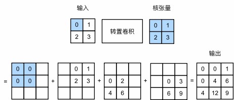
基本操作 设步幅为1且没有填充,假设有一个$n_h \times n_w$的输入张量和一个$k_h \times k_w$的卷积核,以步幅为1滑动卷积核窗口,每行$n_w$次,每列$n_h$次,共产生$n_h n_w$个中间结果,每个中间结果都是一个$(n_h + k_h - 1) \times (n_w + k_w - 1)$的张量,初始化为0
输入张量中的每个元素都要乘以卷积核,从而使所得的$k_h \times k_w$张量替换中间张量的一部分,每个中间张量被替换部分的位置与输入张量中元素的位置相对应。最后,所有中间结果相加以获得最终结果
可以对输入矩阵X和卷积核矩阵K实现基本的转置卷积运算trans_conv
1
2
3
4
5
6
7
def trans_conv (X, K ): h, w = K.shape Y = torch.zeros((X.shape[0 ] + h - 1 , X.shape[1 ] + w - 1 )) for i in range (X.shape[0 ]): for j in range (X.shape[1 ]): Y[i: i + h, j: j + w] += X[i, j] * K return Y
与通过卷积核“减少”输入元素的常规卷积相比,转置卷积通过卷积核“广播”输入元素,从而产生大于输入的输出
当输入X和卷积核K都是四维张量时,可以使用高级API获得相同的结果
1
2
3
tconv = nn.ConvTranspose2d( in_channels, out_channels, kernel_size, stride=1 , padding=0 , bias=True )
参数
含义
in_channels输入通道数(输入特征图的深度)
out_channels输出通道数(输出特征图的深度)
kernel_size卷积核大小(单个数(3)或元组(3,3))
stride步幅(控制上采样扩大倍数),默认1
padding对输出边缘进行裁剪
bias是否学习偏置项,默认True
1
2
3
4
5
6
X = torch.tensor([[0.0 , 1.0 ], [2.0 , 3.0 ]]) K = torch.tensor([[0.0 , 1.0 ], [2.0 , 3.0 ]]) X, K = X.reshape(1 , 1 , 2 , 2 ), K.reshape(1 , 1 , 2 , 2 ) tconv = nn.ConvTranspose2d(1 , 1 , kernel_size=2 , bias=False ) tconv.weight.data = K tconv(X)
1
2
3
tensor([[[[ 0., 0., 1.], [ 0., 4., 6.], [ 4., 12., 9.]]]], grad_fn=<ConvolutionBackward0>)
填充、步幅和多通道 与常规卷积不同,在转置卷积中,填充被应用于输出(常规卷积将填充应用于输入)
当将高和宽两侧的填充数指定为1时,转置卷积的输出中将删除第一和最后的行与列
1
2
3
tconv = nn.ConvTranspose2d(1 , 1 , kernel_size=2 , padding=1 , bias=False ) tconv.weight.data = K tconv(X)
1 tensor([[[[4.]]]], grad_fn=<ConvolutionBackward0>)
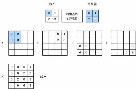
在转置卷积中,步幅被指定为中间结果(输出),而不是输入,使用相同输入和卷积核张量,将步幅从1更改为2会增加中间张量的高和权重,因此输出张量为:
1
2
3
tconv = nn.ConvTranspose2d(1 , 1 , kernel_size=2 , stride=2 , bias=False ) tconv.weight.data = K tconv(X)
1
2
3
4
tensor([[[[0., 0., 0., 1.], [0., 0., 2., 3.], [0., 2., 0., 3.], [4., 6., 6., 9.]]]], grad_fn=<ConvolutionBackward0>)
对于多个输入和输出通道,转置卷积与常规卷积以相同方式运作
假设输入有$c_i$个通道,且转置卷积为每个输入通道分配了一个$k_h\times k_w$的卷积核张量,当指定多个输出通道时,每个输出通道将有一个$c_i\times k_h\times k_w$的卷积核
卷积核参数的整体形状是(out_channels, in_channels, kh, kw)
卷积和转置卷积之间存在反向关系,如果参数(kernel、stride、padding)设得对称,那么转置卷积的输出形状就能还原成卷积的输入形状
1
2
3
4
X = torch.rand(size=(1 , 10 , 16 , 16 )) conv = nn.Conv2d(10 , 20 , kernel_size=5 , padding=2 , stride=3 ) tconv = nn.ConvTranspose2d(20 , 10 , kernel_size=5 , padding=2 , stride=3 ) tconv(conv(X)).shape == X.shape
与矩阵变换的联系 卷积其实就是一种矩阵乘法,假设输入矩阵为 X = torch.arange(9).reshape(3,3)
卷积核为 K = torch.tensor([[1.0, 2.0], [3.0, 4.0]])
普通卷积相当于在X上滑动这个小窗口,不断做“乘加”运算,可以把这个滑动过程,展开成矩阵乘法
构造一个稀疏矩阵 W,它包含了卷积核的权重
1 2 3 4 5 W = [1 2 0 3 4 0 0 0 0] [0 1 2 0 3 4 0 0 0] [0 0 0 1 2 0 3 4 0] [0 0 0 0 1 2 0 3 4]
W 的每一行代表卷积核 K 在图像上滑动到的一个位置
torch.matmul(W, X) 就能得到卷积的输出(展平形式),reshape就得到了卷积的输出矩阵,所以在数学上反卷积(或者说转置卷积)自然就是把这个乘法反过来
也就是用转置矩阵来做乘法
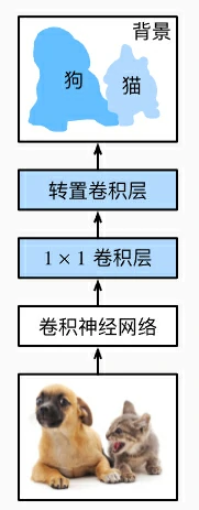
全卷积网络 语义分割是对图像中的每个像素分类,**全卷积网络(fully convolutional network,FCN)**采用卷积神经网络实现了从图像像素到像素类别的变换(Long et al. , 2015),与之前不一样的是全卷积网络通过转置卷积,将中间层特征图的高和宽变换回输入图像的尺寸
构造模型 全卷积网络先使用卷积神经网络抽取图像特征,然后通过1×1卷积层将通道数变换为类别个数,最后通过转置卷积层将特征图的高和宽变换为输入图像的尺寸,因此模型输出与输入图像的高和宽相同,且最终输出通道包含了该空间位置像素的类别预测
使用在ImageNet数据集上预训练的ResNet-18模型来提取图像特征,并将该网络记为pretrained_net
ResNet-18模型的最后几层包括全局平均汇聚层和全连接层,然而全卷积网络中不需要它们
1 pretrained_net = torchvision.models.resnet18(pretrained=True )
创建一个全卷积网络net,它复制了ResNet-18中大部分的预训练层,除了最后的全局平均汇聚层和最接近输出的全连接层
1 net = nn.Sequential(*list (pretrained_net.children())[:-2 ])
给定高度为320和宽度为480的输入,net的前向传播将输入的高和宽减小至原来的1/32,即10和15
1 2 X = torch.rand(size=(1 , 3 , 320 , 480 )) net(X).shape
1 torch.Size([1, 512, 10, 15])
接下来使用1×1卷积层将输出通道数转换为Pascal VOC2012数据集的类数(21类),最后需要将特征图的高度和宽度增加32倍,从而将其变回输入图像的高和宽
根据公式
经验公式:步幅为$s$,填充为$s/2$(如果整除),卷积核的高和宽为$2s$,这样转置卷积核使得输入放大$s$倍
1 2 3 4 num_classes = 21 net.add_module('final_conv' , nn.Conv2d(512 , num_classes, kernel_size=1 )) net.add_module('transpose_conv' , nn.ConvTranspose2d(num_classes, num_classes, kernel_size=64 , padding=16 , stride=32 ))
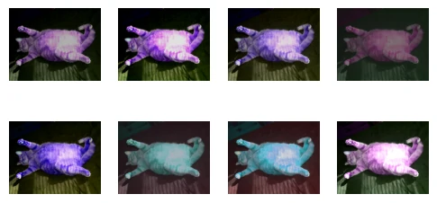
初始化转置卷积层 图像放大通过上采样(upsampling) ,**双线性插值(bilinear interpolation)**是常用的上采样方法之一,它也经常用于初始化转置卷积层
假设给定输入图像,想要计算上采样输出图像上的每个像素
将输出图像的坐标$(x,y)$映射到输入图像的坐标$(x’,y’)$,根据输入与输出的尺寸之比来映射
在输入图像上找到离坐标$(x’,y’)$最近的4个像素
输出图像在坐标$(x,y)$上的像素依据输入图像上这4个像素及其与$(x’,y’)$的相对距离来计算
双线性插值的上采样可以通过转置卷积层实现,内核由以下bilinear_kernel函数构造
1 2 3 4 5 6 7 8 9 10 11 12 13 14 15 16 17 18 19 def bilinear_kernel (in_channels, out_channels, kernel_size ): """生成一个卷积核的权重张量,值是双线性插值滤波器的系数""" factor = (kernel_size + 1 ) // 2 if kernel_size % 2 == 1 : center = factor - 1 else : center = factor - 0.5 og = (torch.arange(kernel_size).reshape(-1 , 1 ), torch.arange(kernel_size).reshape(1 , -1 )) filt = (1 - torch.abs (og[0 ] - center) / factor) * \ (1 - torch.abs (og[1 ] - center) / factor) weight = torch.zeros((in_channels, out_channels, kernel_size, kernel_size)) weight[range (in_channels), range (out_channels), :, :] = filt return weight
构造一个将输入的高和宽放大2倍的转置卷积层,并将其卷积核用bilinear_kernel函数初始化
1 2 3 conv_trans = nn.ConvTranspose2d(3 , 3 , kernel_size=4 , padding=1 , stride=2 , bias=False ) conv_trans.weight.data.copy_(bilinear_kernel(3 , 3 , 4 ));
读取图像X,将上采样的结果记作Y,为了打印图像,需要调整通道维的位置
1 2 3 4 img = torchvision.transforms.ToTensor()(Image.open ('imgs/catdog.jpg' )) X = img.unsqueeze(0 ) Y = conv_trans(X) out_img = Y[0 ].permute(1 , 2 , 0 ).detach()
可以看到,转置卷积层将图像的高和宽分别放大了2倍,除了坐标刻度不同,双线性插值放大的图像和原图看上去没什么两样
1 2 3 print ('input image shape:' , img.permute(1 , 2 , 0 ).shape)print ('output image shape:' , out_img.shape)plt.imshow(out_img);
1 2 input image shape: torch.Size([561, 728, 3]) output image shape: torch.Size([1122, 1456, 3])
全卷积网络用双线性插值的上采样初始化转置卷积层(稳定、快速收敛),对于1×1卷积层使用Xavier初始化参数
1 2 W = bilinear_kernel(num_classes, num_classes, 64 ) net.transpose_conv.weight.data.copy_(W);
读取数据集 用Pascal VOC2012语义分割读取数据集,指定随机裁剪的输出图像的形状为$320\times 480$,高宽都可被32整除
1 2 batch_size, crop_size = 32 , (320 , 480 ) train_iter, test_iter = load_data_voc(batch_size, crop_size)
1 2 read 1114 examples read 1078 examples
训练 可以训练全卷积网络了,这里的损失函数和准确率计算与图像分类中的并没有本质上的不同,因为使用转置卷积层的通道来预测像素的类别,所以需要在损失计算中指定通道维,此外,模型基于每个像素的预测类别是否正确来计算准确率
1 2 3 4 5 6 7 8 def loss (inputs, targets ): """ 等价写法: per_pixel_loss = F.cross_entropy(inputs, targets, reduction='none') # 每像素累计 per_image_loss = per_pixel_loss.mean(dim=(1, 2)) # 每图片平均 """ return F.cross_entropy(inputs, targets, reduction='none' ).mean(1 ).mean(1 )
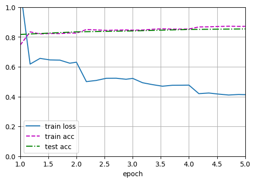
1 2 3 num_epochs, lr, wd, devices = 5 , 0.001 , 1e-3 , try_all_gpus() trainer = torch.optim.SGD(net.parameters(), lr=lr, weight_decay=wd) train_ch13(net, train_iter, test_iter, loss, trainer, num_epochs, devices)
1 2 3 4 5 epoch 1, loss 1.128, acc 0.745, test acc 0.817, time 27.11 sec epoch 2, loss 0.631, acc 0.825, test acc 0.834, time 20.57 sec epoch 3, loss 0.522, acc 0.846, test acc 0.840, time 20.31 sec epoch 4, loss 0.477, acc 0.853, test acc 0.850, time 21.17 sec epoch 5, loss 0.413, acc 0.871, test acc 0.854, time 20.96 sec
1 2 loss 0.413, train acc 0.871, test acc 0.854 82.4 examples/sec on [device(type='cuda', index=0)]
预测 在预测时,需要将输入图像在各个通道做标准化,并转成卷积神经网络所需要的四维输入格式
1 2 3 4 def predict (img ): X = test_iter.dataset.normalize_image(img).unsqueeze(0 ) pred = net(X.to(devices[0 ])).argmax(dim=1 ) return pred.reshape(pred.shape[1 ], pred.shape[2 ])
为了可视化预测的类别给每个像素,将预测类别映射回它们在数据集中的标注颜色
1 2 3 4 def label2image (pred ): colormap = torch.tensor(d2l.VOC_COLORMAP, device=devices[0 ]) X = pred.long() return colormap[X, :]
测试数据集中的图像大小和形状各异,由于模型使用了步幅为32的转置卷积层,因此当输入图像的高或宽无法被32整除时,转置卷积层输出的高或宽会与输入图像的尺寸有偏差
为了解决这个问题,可以在图像中截取多块高和宽为32的整数倍的矩形区域,并分别对这些区域中的像素做前向传播
这些区域的并集需要完整覆盖输入图像,当一个像素被多个区域所覆盖时,它在不同区域前向传播中转置卷积层输出的平均值可以作为softmax运算的输入,从而预测类别
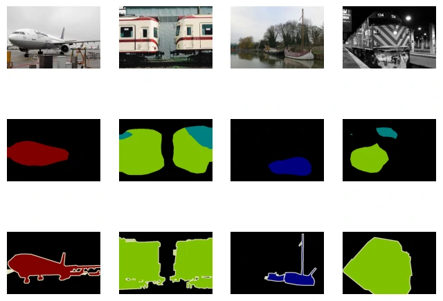
为简单起见,只读取几张较大的测试图像,并从图像的左上角开始截取形状为320×480的区域用于预测
对于这些测试图像,逐一打印它们截取的区域,再打印预测结果,最后打印标注的类别
1 2 3 4 5 6 7 8 9 10 11 12 13 14 15 voc_dir = download_extract('voc2012' , 'VOCdevkit/VOC2012' ) test_images, test_labels = read_voc_images(voc_dir, False ) n, imgs = 4 , [] for i in range (n): crop_rect = (0 , 0 , 320 , 480 ) X = torchvision.transforms.functional.crop(test_images[i], *crop_rect) pred = label2image(predict(X)) imgs += [X.permute(1 ,2 ,0 ), pred.cpu(), torchvision.transforms.functional.crop( test_labels[i], *crop_rect).permute(1 ,2 ,0 )] show_images(imgs[::3 ] + imgs[1 ::3 ] + imgs[2 ::3 ], 3 , n, scale=2 );
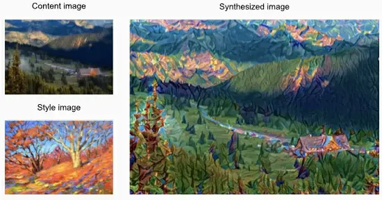
风格迁移 使用卷积神经网络,自动将一个图像中的风格应用在另一图像之上,即风格迁移(style transfer)
需要两张输入图像:一张是内容图像,另一张是风格图像,将使用神经网络修改内容图像,使其在风格上接近风格图像
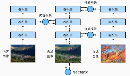
方法 首先,初始化合成图像(通常用内容图像当起点),这张图就是唯一需要更新的变量
然后,选择一个已经训练好的卷积神经网络(比如 VGG),模型参数在训练中无须更新,它只是被拿来当作特征提取器,可以选择其中某些层的输出作为内容特征或风格特征
图中选取的预训练的神经网络含有3个卷积层,其中第二层输出内容特征,第一层和第三层输出风格特征
通过前向传播(实线箭头方向)计算风格迁移的损失函数,并通过反向传播(虚线箭头方向)迭代模型参数,即不断更新合成图像
风格迁移常用的损失函数由3部分组成:
内容损失使合成图像与内容图像在内容特征上接近
风格损失使合成图像与风格图像在风格特征上接近
全变分损失则有助于减少合成图像中的噪点
当模型训练结束时,输出风格迁移的模型参数,即得到最终的合成图像
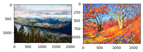
读取内容和风格图像,从打印出的图像坐标轴可以看出,它们的尺寸并不一样
预处理和后处理 定义图像的预处理函数和后处理函数,预处理函数preprocess对输入图像在RGB三个通道分别做标准化,并将结果变换成卷积神经网络接受的输入格式,后处理函数postprocess则将输出图像中的像素值还原回标准化之前的值
由于图像打印函数要求每个像素的浮点数值在0~1之间,对小于0和大于1的值分别取0和1
1 2 3 4 5 6 7 8 9 10 11 12 13 14 15 16 17 rgb_mean = torch.tensor([0.485 , 0.456 , 0.406 ]) rgb_std = torch.tensor([0.229 , 0.224 , 0.225 ]) def preprocess (img, image_shape ): transforms = torchvision.transforms.Compose([ torchvision.transforms.Resize(image_shape), torchvision.transforms.ToTensor(), torchvision.transforms.Normalize(mean=rgb_mean, std=rgb_std)]) return transforms(img).unsqueeze(0 ) def postprocess (img ): img = img[0 ].to(rgb_std.device) img = torch.clamp(img.permute(1 , 2 , 0 ) * rgb_std + rgb_mean, 0 , 1 ) return torchvision.transforms.ToPILImage()(img.permute(2 , 0 , 1 ))
抽取图像特征 使用基于ImageNet数据集预训练的VGG-19模型来抽取图像特征
1 pretrained_net = torchvision.models.vgg19(pretrained=True )
1 2 3 4 5 6 7 8 9 10 11 12 13 14 15 16 17 18 19 20 21 22 23 24 25 26 27 28 29 30 31 32 33 34 35 36 37 38 39 40 41 42 43 44 45 46 47 48 49 50 51 VGG( (features): Sequential( (0): Conv2d(3, 64, kernel_size=(3, 3), stride=(1, 1), padding=(1, 1)) (1): ReLU(inplace=True) (2): Conv2d(64, 64, kernel_size=(3, 3), stride=(1, 1), padding=(1, 1)) (3): ReLU(inplace=True) (4): MaxPool2d(kernel_size=2, stride=2, padding=0, dilation=1, ceil_mode=False) (5): Conv2d(64, 128, kernel_size=(3, 3), stride=(1, 1), padding=(1, 1)) (6): ReLU(inplace=True) (7): Conv2d(128, 128, kernel_size=(3, 3), stride=(1, 1), padding=(1, 1)) (8): ReLU(inplace=True) (9): MaxPool2d(kernel_size=2, stride=2, padding=0, dilation=1, ceil_mode=False) (10): Conv2d(128, 256, kernel_size=(3, 3), stride=(1, 1), padding=(1, 1)) (11): ReLU(inplace=True) (12): Conv2d(256, 256, kernel_size=(3, 3), stride=(1, 1), padding=(1, 1)) (13): ReLU(inplace=True) (14): Conv2d(256, 256, kernel_size=(3, 3), stride=(1, 1), padding=(1, 1)) (15): ReLU(inplace=True) (16): Conv2d(256, 256, kernel_size=(3, 3), stride=(1, 1), padding=(1, 1)) (17): ReLU(inplace=True) (18): MaxPool2d(kernel_size=2, stride=2, padding=0, dilation=1, ceil_mode=False) (19): Conv2d(256, 512, kernel_size=(3, 3), stride=(1, 1), padding=(1, 1)) (20): ReLU(inplace=True) (21): Conv2d(512, 512, kernel_size=(3, 3), stride=(1, 1), padding=(1, 1)) (22): ReLU(inplace=True) (23): Conv2d(512, 512, kernel_size=(3, 3), stride=(1, 1), padding=(1, 1)) (24): ReLU(inplace=True) (25): Conv2d(512, 512, kernel_size=(3, 3), stride=(1, 1), padding=(1, 1)) (26): ReLU(inplace=True) (27): MaxPool2d(kernel_size=2, stride=2, padding=0, dilation=1, ceil_mode=False) (28): Conv2d(512, 512, kernel_size=(3, 3), stride=(1, 1), padding=(1, 1)) (29): ReLU(inplace=True) (30): Conv2d(512, 512, kernel_size=(3, 3), stride=(1, 1), padding=(1, 1)) (31): ReLU(inplace=True) (32): Conv2d(512, 512, kernel_size=(3, 3), stride=(1, 1), padding=(1, 1)) (33): ReLU(inplace=True) (34): Conv2d(512, 512, kernel_size=(3, 3), stride=(1, 1), padding=(1, 1)) (35): ReLU(inplace=True) (36): MaxPool2d(kernel_size=2, stride=2, padding=0, dilation=1, ceil_mode=False) ) (avgpool): AdaptiveAvgPool2d(output_size=(7, 7)) (classifier): Sequential( (0): Linear(in_features=25088, out_features=4096, bias=True) (1): ReLU(inplace=True) (2): Dropout(p=0.5, inplace=False) (3): Linear(in_features=4096, out_features=4096, bias=True) (4): ReLU(inplace=True) (5): Dropout(p=0.5, inplace=False) (6): Linear(in_features=4096, out_features=1000, bias=True) ) )
为了抽取图像的内容特征和风格特征,可以选择VGG网络中某些层的输出,一般来说,越靠近输入层,越容易抽取图像的细节信息,反之,则越容易抽取图像的全局信息
为了避免合成图像过多保留内容图像的细节,选择VGG较靠近输出的层,即内容层,来输出图像的内容特征
还从VGG中选择不同层的输出来匹配局部和全局的风格,这些图层也称为风格层
VGG网络使用了5个卷积块,选择第四卷积块的最后一个卷积层作为内容层,选择每个卷积块的第一个卷积层作为风格层
这些层的索引可以通过打印pretrained_net实例获取
1 style_layers, content_layers = [0 , 5 , 10 , 19 , 28 ], [25 ]
使用VGG层抽取特征时,只需要用到从输入层到最靠近输出层的内容层或风格层之间的所有层
下面构建一个新的网络net,它只保留需要用到的VGG的所有层
1 2 net = nn.Sequential(*[pretrained_net.features[i] for i in range (max (content_layers + style_layers) + 1 )])
给定输入X,如果简单地调用前向传播net(X),只能获得最后一层的输出,由于还需要中间层的输出,因此这里逐层计算,并保留内容层和风格层的输出
1 2 3 4 5 6 7 8 9 10 def extract_features (X, content_layers, style_layers ): contents = [] styles = [] for i in range (len (net)): X = net[i](X) if i in style_layers: styles.append(X) if i in content_layers: contents.append(X) return contents, styles
定义两个函数:get_contents函数对内容图像抽取内容特征; get_styles函数对风格图像抽取风格特征
因为在训练时无须改变预训练的VGG的模型参数,所以可以在训练开始之前就提取出内容特征和风格特征
由于合成图像是风格迁移所需迭代的模型参数,只能在训练过程中通过调用extract_features函数来抽取合成图像的内容特征和风格特征
1 2 3 4 5 6 7 8 9 def get_contents (image_shape, device ): content_X = preprocess(content_img, image_shape).to(device) contents_Y, _ = extract_features(content_X, content_layers, style_layers) return content_X, contents_Y def get_styles (image_shape, device ): style_X = preprocess(style_img, image_shape).to(device) _, styles_Y = extract_features(style_X, content_layers, style_layers) return style_X, styles_Y
定义损失函数 风格迁移的损失函数,它由内容损失、风格损失和全变分损失3部分组成
内容损失 与线性回归中的损失函数类似,内容损失通过平方误差函数衡量合成图像与内容图像在内容特征上的差异
平方误差函数的两个输入均为extract_features函数计算所得到的内容层的输出
1 2 3 4 def content_loss (Y_hat, Y ): return torch.square(Y_hat - Y.detach()).mean()
风格损失 风格损失与内容损失类似,也通过平方误差函数衡量合成图像与风格图像在风格上的差异
为了表达风格层输出的风格,先通过extract_features函数计算风格层的输出
假设该输出的样本数为1,通道数为$c$,高和宽分别为$h$和$w$,可以将此输出转换为矩阵$\mathbf X$,其有$c$行和$hw$列,这个矩阵可以被看作由$c$个长度为$hw$的向量$\mathbf x_1, \ldots, \mathbf x_c$,组合而成的,每个向量代表不同通道上的风格特征
这些向量的格拉姆矩阵 $\mathbf X\mathbf X^\top \in \mathbb{R}^{c \times c}$,$i$行$j$列的元素$x_{ij}$即向量$x_i$和$x_j$的内积,表达了通道$i$和$j$上风格特征的相关性,用这样的格拉姆矩阵来表达风格层输出的风格
当$hw$的值较大时,格拉姆矩阵中的元素容易出现较大的值,此外格拉姆矩阵的高和宽皆为通道数$c$
为了让风格损失不受这些值的大小影响,下面定义的gram函数将格拉姆矩阵除以了矩阵中元素的个数$chw$
1 2 3 4 def gram (X ): num_channels, n = X.shape[1 ], X.numel() // X.shape[1 ] X = X.reshape((num_channels, n)) return torch.matmul(X, X.T) / (num_channels * n)
自然地,风格损失的平方误差函数的两个格拉姆矩阵输入分别基于合成图像与风格图像的风格层输出
这里假设基于风格图像的格拉姆矩阵gram_Y已经预先计算好了
1 2 def style_loss (Y_hat, gram_Y ): return torch.square(gram(Y_hat) - gram_Y.detach()).mean()
全变分损失 合成图像里面有大量高频噪点,即有特别亮或者特别暗的颗粒像素,一种常见的去噪方法是全变分去噪(total variation denoising)
假设$x_{i, j}$表示坐标$(i, j)$处的像素值,降低全变分损失
1 2 3 4 def tv_loss (Y_hat ): return 0.5 * (torch.abs (Y_hat[:, :, 1 :, :] - Y_hat[:, :, :-1 , :]).mean() + torch.abs (Y_hat[:, :, :, 1 :] - Y_hat[:, :, :, :-1 ]).mean())
损失函数 风格转移的损失函数是内容损失、风格损失和总变化损失的加权和,通过调节这些权重超参数,可以权衡合成图像在保留内容、迁移风格以及去噪三方面的相对重要性
1 2 3 4 5 6 7 8 9 10 11 12 content_weight, style_weight, tv_weight = 1 , 1e3 , 10 def compute_loss (X, contents_Y_hat, styles_Y_hat, contents_Y, styles_Y_gram ): contents_l = [content_loss(Y_hat, Y) * content_weight for Y_hat, Y in zip ( contents_Y_hat, contents_Y)] styles_l = [style_loss(Y_hat, Y) * style_weight for Y_hat, Y in zip ( styles_Y_hat, styles_Y_gram)] tv_l = tv_loss(X) * tv_weight l = sum (10 * styles_l + contents_l + [tv_l]) return contents_l, styles_l, tv_l, l
初始化合成图像 可以定义一个简单的模型SynthesizedImage,并将合成的图像视为模型参数,模型的前向传播只需返回模型参数即可
1 2 3 4 5 6 7 class SynthesizedImage (nn.Module): def __init__ (self, img_shape, **kwargs ): super ().__init__(**kwargs) self .weight = nn.Parameter(torch.rand(*img_shape)) def forward (self ): return self .weight
定义get_inits函数,该函数创建了合成图像的模型实例,并将其初始化为图像X,风格图像在各个风格层的格拉姆矩阵styles_Y_gram将在训练前预先计算好
1 2 3 4 5 6 7 8 9 def get_inits (X, device, lr, styles_Y ): gen_img = SynthesizedImage(X.shape).to(device) gen_img.weight.data.copy_(X.data) trainer = torch.optim.Adam(gen_img.parameters(), lr=lr) styles_Y_gram = [gram(Y) for Y in styles_Y] return gen_img(), styles_Y_gram, trainer
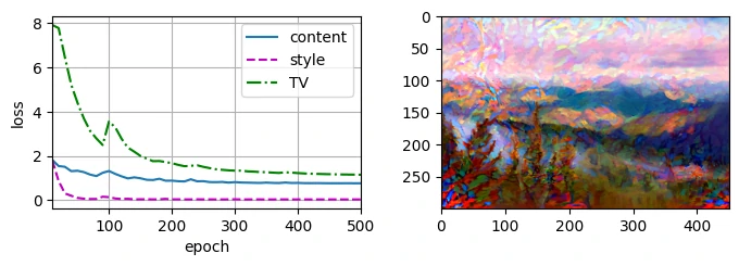
训练模型 在训练模型进行风格迁移时,不断抽取合成图像的内容特征和风格特征,然后计算损失函数,下面定义了训练循环
1 2 3 4 5 6 7 8 9 10 11 12 13 14 15 16 17 18 19 20 21 22 23 24 25 26 def train (X, contents_Y, styles_Y, device, lr, num_epochs, lr_decay_epoch ): X, styles_Y_gram, trainer = get_inits(X, device, lr, styles_Y) scheduler = torch.optim.lr_scheduler.StepLR(trainer, lr_decay_epoch, 0.8 ) animator = Animator(xlabel='epoch' , ylabel='loss' , xlim=[10 , num_epochs], legend=['content' , 'style' , 'TV' ], ncols=2 , figsize=(7 , 2.5 )) for epoch in range (num_epochs): trainer.zero_grad() contents_Y_hat, styles_Y_hat = extract_features( X, content_layers, style_layers) contents_l, styles_l, tv_l, l = compute_loss( X, contents_Y_hat, styles_Y_hat, contents_Y, styles_Y_gram) l.backward() trainer.step() scheduler.step() if (epoch + 1 ) % 10 == 0 : animator.axes[1 ].imshow(postprocess(X)) animator.add(epoch + 1 , [float (sum (contents_l)), float (sum (styles_l)), float (tv_l)]) return X
1 2 3 4 5 6 content_weight, style_weight, tv_weight = 1 , 1e3 , 10 device, image_shape = try_gpu(), (300 , 450 ) net = net.to(device) content_X, contents_Y = get_contents(image_shape, device) _, styles_Y = get_styles(image_shape, device) output = train(content_X, contents_Y, styles_Y, device, 0.3 , 500 , 50 )
可以看到,合成图像保留了内容图像的风景和物体,并同时迁移了风格图像的色彩
例如,合成图像具有与风格图像中一样的色彩块,其中一些甚至具有画笔笔触的细微纹理
实战 Kaggle 比赛:图像分类 (CIFAR-10) 之前一直用深度学习框架的高级API直接获取张量格式的图像数据集;在实践中,图像数据集通常以图像文件的形式出现
将从原始图像文件开始,然后逐步组织、读取并将它们转换为张量格式
导入竞赛所需的包和模块
1 2 3 4 5 6 7 8 import collectionsimport mathimport osimport shutil import pandas as pdimport torchimport torchvisionfrom torch import nn
获取并组织数据集 比赛数据集分为训练集和测试集,其中训练集包含50000张、测试集包含300000张图像
在测试集中,10000张图像将被用于评估,而剩下的290000张图像将不会被进行评估,包含它们只是为了防止手动标记测试集并提交标记结果
两个数据集中的图像都是png格式,高度和宽度均为32像素并有三个颜色通道(RGB)
这些图片共涵盖10个类别:飞机、汽车、鸟类、猫、鹿、狗、青蛙、马、船和卡车
下载数据集 登录Kaggle后可以点击显示的CIFAR-10图像分类竞赛网页上的“Data”选项卡,然后单击“Download All”按钮下载数据集
在../data中解压下载的文件并在其中解压缩train.7z和test.7z后,在以下路径中可以找到整个数据集:
../data/cifar-10/train/[1-50000].png../data/cifar-10/test/[1-300000].png../data/cifar-10/trainLabels.csv../data/cifar-10/sampleSubmission.csv
为了便于入门,提供包含前1000个训练图像和5个随机测试图像的数据集的小规模样本
要使用Kaggle竞赛的完整数据集,需要将以下demo变量设置为False
1 2 3 4 5 6 7 8 9 10 11 DATA_HUB = dict () DATA_URL = 'http://d2l-data.s3-accelerate.amazonaws.com/' DATA_HUB['cifar10_tiny' ] = ( DATA_URL + 'kaggle_cifar10_tiny.zip' , '2068874e4b9a9f0fb07ebe0ad2b29754449ccacd' ) demo = True if demo: data_dir = download_extract('cifar10_tiny' ) else : data_dir = '../data/cifar-10/'
整理数据集 需要整理数据集来训练和测试模型,首先用以下函数读取CSV文件中的标签,它返回一个字典,该字典将文件名中不带扩展名的部分映射到其标签
1 2 3 4 5 6 7 def read_csv_labels (fname ): """读取fname来给标签字典返回一个文件名""" with open (fname, 'r' ) as f: lines = f.readlines()[1 :] tokens = [l.rstrip().split(',' ) for l in lines] return dict (((name, label) for name, label in tokens))
1 2 3 labels = read_csv_labels(os.path.join(data_dir, 'trainLabels.csv')) print('# 训练样本 :', len(labels)) print('# 类别 :', len(set(labels.values())))
定义reorg_train_valid函数来将验证集从原始的训练集中拆分出来,此函数中的参数valid_ratio是验证集中的样本数与原始训练集中的样本数之比
组织数据集后,同类别的图像将被放置在同一文件夹下
1 2 3 4 5 6 7 8 9 10 11 12 13 14 15 16 17 18 19 20 21 22 23 24 25 26 27 28 29 30 31 32 33 34 35 36 37 38 39 40 41 42 43 44 45 46 47 48 def copyfile (filename, target_dir ): """将文件复制到目标目录""" os.makedirs(target_dir, exist_ok=True ) shutil.copy(filename, target_dir) def reorg_train_valid (data_dir, labels, valid_ratio ): """将验证集从原始训练集中拆分出来 参数: data_dir:数据集的主目录路径 labels:字典,键是图片文件名(不带后缀),值是类别名称 valid_ratio:验证集比例(例如 0.1 表示 10% 数据作为验证集) 返回: n_valid_per_label:每个类别划入验证集的样本数量 """ n = collections.Counter(labels.values()).most_common()[-1 ][1 ] n_valid_per_label = max (1 , math.floor(n * valid_ratio)) label_count = {} for train_file in os.listdir(os.path.join(data_dir, 'train' )): label = labels[train_file.split('.' )[0 ]] fname = os.path.join(data_dir, 'train' , train_file) copyfile(fname, os.path.join(data_dir, 'train_valid_test' , 'train_valid' , label)) if label not in label_count or label_count[label] < n_valid_per_label: copyfile(fname, os.path.join(data_dir, 'train_valid_test' , 'valid' , label)) label_count[label] = label_count.get(label, 0 ) + 1 else : copyfile(fname, os.path.join(data_dir, 'train_valid_test' , 'train' , label)) return n_valid_per_label
reorg_test函数用来在预测期间整理测试集,以方便读取
1 2 3 4 5 6 def reorg_test (data_dir ): """在预测期间整理测试集,以方便读取""" for test_file in os.listdir(os.path.join(data_dir, 'test' )): copyfile(os.path.join(data_dir, 'test' , test_file), os.path.join(data_dir, 'train_valid_test' , 'test' , 'unknown' ))
最后使用一个函数来调用前面定义的函数read_csv_labels、reorg_train_valid和reorg_test
1 2 3 4 def reorg_cifar10_data (data_dir, valid_ratio ): labels = read_csv_labels(os.path.join(data_dir, 'trainLabels.csv' )) reorg_train_valid(data_dir, labels, valid_ratio) reorg_test(data_dir)
在这里只将样本数据集的批量大小设置为32,在实际训练和测试中,应该使用Kaggle竞赛的完整数据集,并将batch_size设置为更大的整数,例如128,将10%的训练样本作为调整超参数的验证集
1 2 3 batch_size = 32 if demo else 128 valid_ratio = 0.1 reorg_cifar10_data(data_dir, valid_ratio)
图像增广 使用图像增广来解决过拟合的问题,在训练中可以随机水平翻转图像,还可以对彩色图像的三个RGB通道执行标准化
1 2 3 4 5 6 7 8 9 10 11 12 13 transform_train = torchvision.transforms.Compose([ torchvision.transforms.Resize(40 ), torchvision.transforms.RandomResizedCrop(32 , scale=(0.64 , 1.0 ), ratio=(1.0 , 1.0 )), torchvision.transforms.RandomHorizontalFlip(), torchvision.transforms.ToTensor(), torchvision.transforms.Normalize([0.4914 , 0.4822 , 0.4465 ], [0.2023 , 0.1994 , 0.2010 ])])
在测试期间只对图像执行标准化,以消除评估结果中的随机性
1 2 3 4 transform_test = torchvision.transforms.Compose([ torchvision.transforms.ToTensor(), torchvision.transforms.Normalize([0.4914 , 0.4822 , 0.4465 ], [0.2023 , 0.1994 , 0.2010 ])])
读取数据集 读取由原始图像组成的数据集,每个样本都包括一张图片和一个标签
1 2 3 4 5 6 7 train_ds, train_valid_ds = [torchvision.datasets.ImageFolder( os.path.join(data_dir, 'train_valid_test' , folder), transform=transform_train) for folder in ['train' , 'train_valid' ]] valid_ds, test_ds = [torchvision.datasets.ImageFolder( os.path.join(data_dir, 'train_valid_test' , folder), transform=transform_test) for folder in ['valid' , 'test' ]]
在训练期间需要指定上面定义的所有图像增广操作,当验证集在超参数调整过程中用于模型评估时,不应引入图像增广的随机性
在最终预测之前,根据训练集和验证集组合而成的训练模型进行训练,以充分利用所有标记的数据
1 2 3 4 5 6 7 8 9 train_iter, train_valid_iter = [torch.utils.data.DataLoader( dataset, batch_size, shuffle=True , drop_last=True ) for dataset in (train_ds, train_valid_ds)] valid_iter = torch.utils.data.DataLoader(valid_ds, batch_size, shuffle=False , drop_last=True ) test_iter = torch.utils.data.DataLoader(test_ds, batch_size, shuffle=False , drop_last=False )
定义模型 使用ResNet18
1 2 3 4 5 6 def get_net (): num_classes = 10 net = resnet18(num_classes, 3 ) return net loss = nn.CrossEntropyLoss(reduction="none" )
定义训练函数 将根据模型在验证集上的表现来选择模型并调整超参数,下面定义了模型训练函数train
1 2 3 4 5 6 7 8 9 10 11 12 13 14 15 16 17 18 19 20 21 22 23 24 25 26 27 28 29 30 31 32 33 34 35 def train (net, train_iter, valid_iter, num_epochs, lr, wd, devices, lr_period, lr_decay ): trainer = torch.optim.SGD(net.parameters(), lr=lr, momentum=0.9 , weight_decay=wd) scheduler = torch.optim.lr_scheduler.StepLR(trainer, lr_period, lr_decay) num_batches, timer = len (train_iter), Timer() legend = ['train loss' , 'train acc' ] if valid_iter is not None : legend.append('valid acc' ) animator = Animator(xlabel='epoch' , xlim=[1 , num_epochs], legend=legend) net = nn.DataParallel(net, device_ids=devices).to(devices[0 ]) for epoch in range (num_epochs): net.train() metric = Accumulator(3 ) for i, (features, labels) in enumerate (train_iter): timer.start() l, acc = train_batch_ch13(net, features, labels, loss, trainer, devices) metric.add(l, acc, labels.shape[0 ]) timer.stop() if (i + 1 ) % (num_batches // 5 ) == 0 or i == num_batches - 1 : animator.add(epoch + (i + 1 ) / num_batches, (metric[0 ] / metric[2 ], metric[1 ] / metric[2 ], None )) if valid_iter is not None : valid_acc = evaluate_accuracy_gpu(net, valid_iter) animator.add(epoch + 1 , (None , None , valid_acc)) scheduler.step() measures = (f'train loss {metric[0 ] / metric[2 ]:.3 f} , ' f'train acc {metric[1 ] / metric[2 ]:.3 f} ' ) if valid_iter is not None : measures += f', valid acc {valid_acc:.3 f} ' print (measures + f'\n{metric[2 ] * num_epochs / timer.sum ():.1 f} ' f' examples/sec on {str (devices)} ' )
训练和验证模型 以下所有超参数都可以调整,比如可以增加周期的数量
当lr_period和lr_decay分别设置为4和0.9时,优化算法的学习速率将在每4个周期乘以0.9,在这里只训练20个周期
1 2 3 4 devices, num_epochs, lr, wd = try_all_gpus(), 20 , 2e-4 , 5e-4 lr_period, lr_decay, net = 4 , 0.9 , get_net() train(net, train_iter, valid_iter, num_epochs, lr, wd, devices, lr_period, lr_decay)
对测试集进行分类并提交结果 1 2 3 4 5 6 7 8 9 10 11 12 net, preds = get_net(), [] train(net, train_valid_iter, None , num_epochs, lr, wd, devices, lr_period, lr_decay) for X, _ in test_iter: y_hat = net(X.to(devices[0 ])) preds.extend(y_hat.argmax(dim=1 ).type (torch.int32).cpu().numpy()) sorted_ids = list (range (1 , len (test_ds) + 1 )) sorted_ids.sort(key=lambda x: str (x)) df = pd.DataFrame({'id' : sorted_ids, 'label' : preds}) df['label' ] = df['label' ].apply(lambda x: train_valid_ds.classes[x]) df.to_csv('submission.csv' , index=False )