OpenCV 是一个功能强大、应用广泛的计算机视觉库,提供了大量的计算机视觉算法和图像处理工具,广泛应用于图像和视频的处理、分析以及机器学习领域
使用pip安装是最简单和直接的方法,只需要在命令行中输入以下命令:
1 pip install opencv-python
安装后导入包:
图像理论 图像在计算机中本质上是以数字矩阵的形式存储的,其核心概念包括像素网格和颜色通道
像素网格:
像素(pixel):图片的最小单元,每个像素有位置(行、列)和颜色值
分辨率:宽×高(例如1920×1080),表示像素矩阵的尺寸
像素矩阵:一张图片在内存里通常就是一个二维或三维数组(矩阵),H行xW列(x3or4通道) ,坐标系通常是左上角为原点(行号向下增大)
颜色与通道:
RGB:最常见,基于人眼感知颜色的方式,每个像素由3个通道(红、绿、蓝)组合成颜色
RGBA:RGB + Alpha(透明度),Alpha 通道决定像素的透明程度
灰度:只有一个通道(亮度),常用公式把 RGB 转成灰度:Y = 0.299 R + 0.587 G + 0.114 B(ITU标准) 0为黑,255为白
CMYK:印刷领域(青、品红、黄、黑),基于减色法
YCbCr:主要用于JPEG,RGB转YCbCr,再对Cb、Cr下采样(4:2:0常见),再做DCT压缩
Pillow/Matplotlib用RGB顺序,OpenCV默认用BGR ,注意转换
位深与数据类型:
常见的存储方式:
格式
压缩方式
是否有损
支持透明度
特点与应用场景
BMP
无
无损
支持
简单直白,文件大
PNG
DEFLATE
无损
支持 Alpha
体积比BMP小
GIF
LZW
无损
1 位透明
支持简单动画,但颜色数少
SVG
XML,可GZIP
无损
支持 Alpha
无限缩放不失真
JPEG
DCT+量化
有损
不支持
照片最常用格式,高压缩比
TIFF
多种
均可
支持
专业图像格式,高位深
WebP
VP8/VP8L压缩
均可
支持 Alpha
压缩比优于JPEG/PNG,Web 常见
代码性能评估 1 2 3 4 5 6 import cv2start = cv2.getTickCount() end = cv2.getTickCount() print ((end - start) / cv2.getTickFrequency())
也可以用 time 模块计时
1
2
3
4
5
6
import timestart = time.clock() end = time.clock() print (end - start)
数据元素少时用 Python 语法,数据元素多时用 Numpy
1 2 3 4 5 6 7 8 x = 10 z = np.uint8([10 ]) start = cv2.getTickCount() y = z*z*z end = cv2.getTickCount() print ((end - start) / cv2.getTickFrequency())
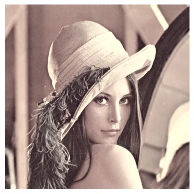
图像基础操作 读取图片 :
1 2 3 4 img = cv2.imread('Lena.bmp' , 0 ) if img is None : print ("Cannot load image" ) exit()
参数1:图片的文件名
参数2:读入方式,省略即采用默认值
cv2.IMREAD_COLOR:彩色图,默认值(1)cv2.IMREAD_GRAYSCALE:灰度图(0)cv2.IMREAD_UNCHANGED:包含透明通道的彩色图(-1)
显示图片 :
1 2 3 cv2.imshow("Lena" ,img) cv2.waitKey(0 )
保存图片 :
1 cv2.imwrite("Lena_gray.bmp" ,img)
可以传入第三个参数:
cv2.IMWRITE_JPEG_QUALITY:jpg 质量控制,取值 0~100,值越大质量越好,默认为 95cv2.IMWRITE_PNG_COMPRESSION:png 质量控制,取值 0~9,值越大压缩比越高,默认为 1
1 2 3 4 cv2.imwrite('img_jpg20.jpg' ,img, [int (cv2.IMWRITE_JPEG_QUALITY), 20 ]) cv2.imwrite('img_jpg100.jpg' ,img, [int (cv2.IMWRITE_JPEG_QUALITY), 100 ]) cv2.imwrite('img_png.png' ,img) cv2.imwrite('img_png9.png' ,img,[int (cv2.IMWRITE_PNG_COMPRESSION),9 ])
图像矩阵 OpenCV读进来的图像是NumPy数组,shape通常是(H, W, C),可以通过img.shape输出
1 2 height, width, channels = img.shape
图像是由像素组成的矩阵,每个像素都有一个或多个值,表示颜色或灰度
OpenCV默认的颜色空间为BGR
1 2 3 4 5 img = cv2.imread("LenaRGB.bmp" ,1 ) px = img[99 ,99 ] print (px) px_blue = img[99 ,99 ,0 ] print (px_blue)
ROI(Region of Interest):利用:,也就是numpy的切片,将图片中的区域裁切出来
1 2 3 4 face = img[239 :388 , 238 :356 ] cv2.imshow("face" ,face) cv2.waitKey(0 )
颜色空间 OpenCV 支持多种颜色空间的转换,通过cv2.cvtColor(img, code)
常用转化code:
cv2.COLOR_BGR2GRAY: BGR彩色 -> 灰度cv2.COLOR_BGR2RGB: BGR彩色 -> RGB彩色(用于Matplotlib等显示)cv2.COLOR_BGR2HSV: BGR彩色 -> HSV(色相、饱和度、亮度)cv2.COLOR_GRAY2BGR: 灰度 -> BGR彩色 (单通道转三通道)
颜色通道的分离与合并:
1 2 3 4 b, g, r = cv2.split(image) merged_image = cv2.merge([b, g, r])
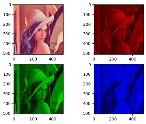
单通道显示:
1 2 3 4 5 6 7 8 9 10 11 12 13 14 15 img = cv2.imread("LenaRGB.bmp" ,1 ) b, g, r = cv2.split(img) zeros = np.zeros_like(b) blue_img = cv2.merge([b, zeros, zeros]) green_img = cv2.merge([zeros, g, zeros]) red_img = cv2.merge([zeros, zeros, r]) plt.subplot(2 ,2 ,1 ) plt.imshow(cv2.cvtColor(img,cv2.COLOR_BGR2RGB)) plt.subplot(2 ,2 ,2 ) plt.imshow(blue_img) plt.subplot(2 ,2 ,3 ) plt.imshow(green_img) plt.subplot(2 ,2 ,4 ) plt.imshow(red_img)
RGB 调色板 首先需要知道如何创建滑动条(滑块最小值固定为0)
1 cv2.createTrackbar(trackbarName, windowName, value, max_value ,call_back)
实现一个 RGB 的调色板:
1 2 3 4 5 6 7 8 9 10 11 12 13 14 15 16 17 18 19 20 21 22 23 def nothing (x ): pass img = np.zeros((300 ,500 ,3 ), np.uint8) cv2.namedWindow("RGB Palette" ) cv2.createTrackbar("R" ,"RGB Palette" , 0 , 255 , nothing) cv2.createTrackbar("G" ,"RGB Palette" , 0 , 255 , nothing) cv2.createTrackbar("B" ,"RGB Palette" , 0 , 255 , nothing) while True : r = cv2.getTrackbarPos("R" , "RGB Palette" ) g = cv2.getTrackbarPos("G" , "RGB Palette" ) b = cv2.getTrackbarPos("B" , "RGB Palette" ) img[:] = [b, g, r] cv2.imshow("RGB Palette" , img) if cv2.waitKey(1 ) & 0xFF == 27 : break cv2.destroyAllWindows()
几何变换 在cv2的函数中输入的一般是(w,h),虽然在numpy输出的shape是(h,w)
仿射变换 cv2.warpAffine():仿射变换是一种保持直线和比例关系的线性几何变换
长度/角度可能变化,但相对位置关系不变
常见的仿射变换包括:缩放、翻转、平移、旋转
1 dst = cv2.warpAffine(img, M, dsize)
其中M是变换矩阵,dsize是输出图像大小(width, height)
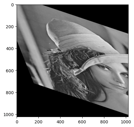
变换矩阵可以通过cv2.getAffineTransform()求得,只需要知道变换前后对应三个点的坐标即可
1 2 3 4 5 6 7 8 img = cv2.imread("Lena.bmp" ) rows, cols = img.shape[:2 ] pts1 = np.float32([[50 , 50 ], [100 , 50 ], [50 , 200 ]]) pts2 = np.float32([[0 , 0 ], [150 , 50 ], [100 , 250 ]]) M = cv2.getAffineTransform(pts1, pts2) dst = cv2.warpAffine(img, M, (cols*2 , rows*2 )) plt.imshow(dst,'gray' )
缩放 cv2.resize():调整图像大小(放大或缩小)
1 2 3 4 5 resized_img = cv2.resize(img, (new_width,new_height)) scale_factor = 0.5 resized_img = cv2.resize(img, None , fx=scale_factor, fy=scale_factor, interpolation=cv2.INTER_AREA)
interpolation(插值方法):
cv2.INTER_LINEAR 双线性(默认,放大推荐)cv2.INTER_AREA 区域插值(缩小推荐)cv2.INTER_CUBIC 三次插值(更平滑,慢)cv2.INTER_NEAREST 最近邻(最快,但可能马赛克)
翻转 cv2.flip():
1 2 flipped_img = cv2.flip(image, flip_code)
平移 使用仿射变换函数cv2.warpAffine()
需要定义一个变换矩阵,$tx ,ty$是向$x$和$y$方向平移的距离,$M=[[1,0,t_x],[0,1,t_y]]$
1 2 3 4 (h, w) = img.shape[:2 ] translation_matrix = np.float32([[1 , 0 , 100 ], [0 , 1 , 50 ]]) shifted_img = cv2.warpAffine(img, translation_matrix, (w, h))
旋转 使用仿射变换函数cv2.warpAffine()
绕某个点旋转,可伴随缩放,也需要定义一个变换矩阵
通过cv2.getRotationMatrix2D()函数来生成这个矩阵,该函数有三个参数
参数1:图片的旋转中心(一般是(w//2,h//2))
参数2:旋转角度(正:逆时针,负:顺时针)
参数3:缩放比例,0.5 表示缩小一半
1 2 3 center = (w//2 , h//2 ) rotation_matrix = cv2.getRotationMatrix2D(center, 45 , 0.5 ) rotated_img = cv2.warpAffine(img, rotation_matrix, (w, h))
图像加减法 相加减两幅图片的形状(高度/宽度/通道数)必须相同
1 2 result = cv2.add(img1, img2) result = cv2.subtract(img1, img2)
numpy中可以直接用 res = img + img1 相加,但这两者的结果并不相同
如果像素值相加后超过255,OpenCV 会自动将其截断为255(注意,必须是二维矩阵)
1 2 3 4 x = np.uint8([[250 ]]) y = np.uint8([[10 ]]) print ("cv2.add:" , cv2.add(x, y)) print ("numpy + :" , x + y)
图像位运算 图像位运算是将两幅图像的每个像素值转为二进制以后进行位操作
图像必须是相同大小和通道数,否则不能直接做按位运算
主要用于二值图像处理 以及掩膜运算 (掩膜mask是对一幅图片进行局部的遮挡)
函数
功能
应用场景
cv2.bitwise_and(img1,img2)按位与操作
掩膜交集
cv2.bitwise_or(img1,img2)按位或操作
掩膜并集
cv2.bitwise_not(img)按位取反操作
反转掩膜
cv2.bitwise_xor(img1,img2)按位异或操作
掩膜并集-交集
利用图片自身按位与 ,掩膜上为255的保留原值,为0的区域置0
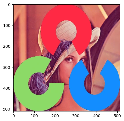
按位与 1 2 3 4 5 6 img1 = cv2.imread("LenaRGB.bmp" , 1 ) img2 = cv2.imread("OpenCV_logo_no_text.png" , 1 ) img2 = cv2.resize(img2,(img1.shape[1 ],img1.shape[0 ])) img2_gray = cv2.cvtColor(img2, cv2.COLOR_BGR2GRAY) plt.imshow(img2_gray, cmap='gray' )
1 2 3 4 5 6 7 8 9 10 11 12 13 14 _, mask = cv2.threshold(img2_gray, 10 , 255 , cv2.THRESH_BINARY) mask_inv = cv2.bitwise_not(mask) img1_bg = cv2.bitwise_and(img1, img1, mask=mask_inv) img2_fg = cv2.bitwise_and(img2, img2, mask=mask) res = cv2.add(img1_bg,img2_fg) res = cv2.cvtColor(res, cv2.COLOR_BGR2RGB) plt.imshow(res)
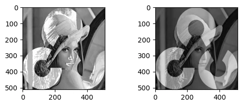
按位或 按位或并不等同于图像叠加
1 2 3 4 5 6 7 8 9 img1 = cv2.imread("Lena.bmp" , 0 ) img2 = cv2.imread("OpenCV_logo_no_text.png" , 0 ) img2 = cv2.resize(img2,(img1.shape[1 ],img1.shape[0 ])) res1 = cv2.bitwise_or(img1, img2) res2 = cv2.addWeighted(img1, 0.5 , img2, 0.5 , 0 ) plt.subplot(2 ,2 ,1 ) plt.imshow(res1, cmap='gray' ) plt.subplot(2 ,2 ,2 ) plt.imshow(res2,cmap='gray' )
图像融合 阿尔法混合(加权混合) 图像混合就是把两张图像的像素值按照一定比例组合
1 2 3 4 5 6 7 8 9 10 11 img1 = cv2.imread("Barbara.bmp" , 0 ) img2 = cv2.imread("Baboon.bmp" , 0 ) img2 = cv2.resize(img2,(img1.shape[1 ],img1.shape[0 ])) for alpha in np.linspace(0 , 1 , 20 ): beta = 1 - alpha blended = cv2.addWeighted(img1, alpha, img2, beta, 0 ) cv2.imshow("Blending" , blended) cv2.waitKey(200 ) cv2.destroyAllWindows()
拉普拉斯金字塔融合 如果直接把两张图拼接,边界很明显:
即使用线性渐变(alpha blending),仍可能出现模糊边界或鬼影
金字塔融合的核心思想:在不同的尺度(分辨率)上融合图像
适合那些既要平滑过渡,又要细节自然的场景,但是会损失细节
图像金字塔有两种:高斯金字塔 和拉普拉斯金字塔
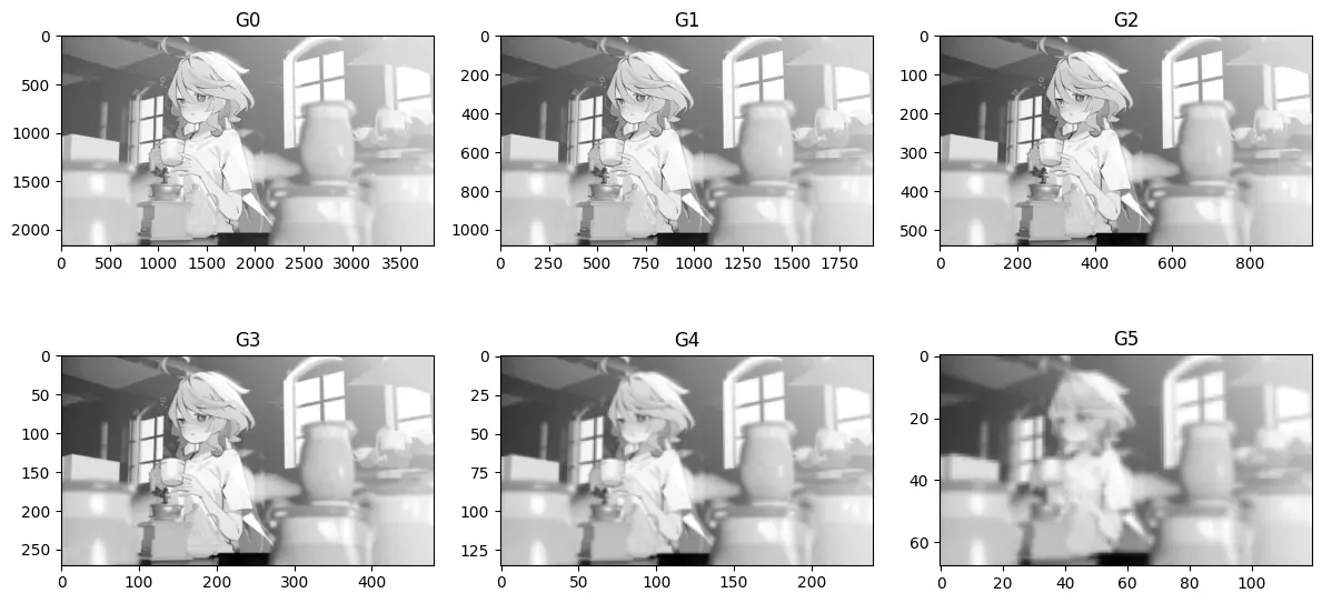
高斯金字塔中较高层中的每个像素都是由其下一层中的5个像素以高斯权重贡献形成的
对于$M\times N$的图像,通过cv.pyrDown()[下采样]变成$M/2\times N/2$,获得金字塔的上层
1 2 3 4 5 6 7 8 9 def generate_gaussian_pyramid (img, level=6 ): G = img.copy() gp = [G] for i in range (level): G = cv2.pyrDown(G) gp.append(G) return gp
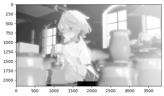
1 2 3 4 5 6 7 8 img = cv2.imread("imgs/funingna.png" , 0 ) gp = generate_gaussian_pyramid(img, level=5 ) plt.figure(figsize=(12 , 6 )) for i in range (len (gp)): plt.subplot(2 ,3 ,i+1 ) plt.imshow(gp[i], cmap='gray' ) plt.title(f"G{i} " ) plt.tight_layout()
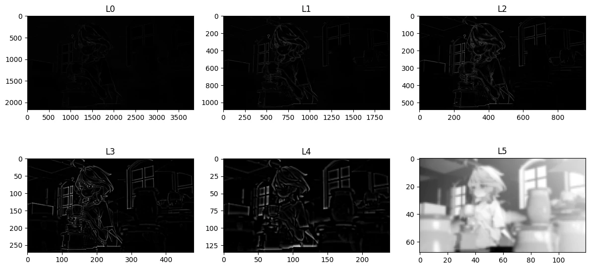
拉普拉斯金字塔由高斯金字塔该层与上层cv.pyrUp()[上采样]之间的差值形成
也可以写成(代码循环常这么写)
1 2 3 4 5 6 7 8 9 10 11 12 def generate_laplacian_pyramid (gp ): N = len (gp) lp = [gp[N-1 ]] for i in range (N-1 ,0 ,-1 ): GE = cv2.pyrUp(gp[i]) GE = cv2.resize(GE,(gp[i-1 ].shape[1 ],gp[i-1 ].shape[0 ])) L = cv2.subtract(gp[i-1 ], GE) lp.append(L) return lp
需要注意的是,由于计算的时候是从Gn开始计算,所以生成的拉普拉斯金字塔列表是反转过来的
1 2 3 4 5 6 7 8 lp = generate_laplacian_pyramid(gp) lp = lp[::-1 ] plt.figure(figsize=(12 , 6 )) for i in range (len (lp)): plt.subplot(2 ,3 ,i+1 ) plt.imshow(lp[i],cmap='gray' ) plt.title(f"L{i} " ) plt.tight_layout()
融合两张图片的拉普拉斯金字塔,获得最终图的拉普拉斯金字塔
1 2 3 4 5 6 7 8 9 10 11 12 13 14 15 16 17 18 19 20 def blend_half (lpA, lpB ): LS = [] for la, lb in zip (lpA, lpB): rows, cols, dpt = la.shape ls = np.hstack((la[:,:cols//2 ], lb[:, cols//2 :])) LS.append(ls) return LS def blend_gradient (lpA, lpB ): LS = [] for la, lb in zip (lpA, lpB): rows, cols, dpt = la.shape mask = np.linspace(1 , 0 , cols).reshape(1 , -1 , 1 ) mask = np.repeat(mask, rows, axis=0 ) ls = la * mask + lb * (1 -mask) LS.append(ls.astype(np.uint8)) return LS
重建图样从最小的高斯图(最高层)开始,逐层往大推
1 2 3 4 5 6 7 8 def reconstruct_from_laplacian (LS ): G = LS[0 ] for i in range (1 , len (LS)): GE = cv2.pyrUp(G) GE = cv2.resize(GE,(LS[i].shape[1 ],LS[i].shape[0 ])) G = cv2.add(GE, LS[i]) return G
因为在生成拉普拉斯金字塔时把Gn放在了列表头部,所以就不需要反转了!
1 2 res = reconstruct_from_laplacian(lp[::-1 ]) plt.imshow(res, cmap='gray' )
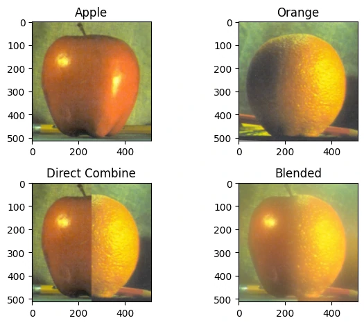
官方demo:苹果+橘子
1 2 3 4 5 6 7 8 9 10 11 12 13 14 15 16 apple = cv2.imread("imgs/apple.jpg" , 1 ) orange = cv2.imread("imgs/orange.jpg" , 1 ) gpA = generate_gaussian_pyramid(apple) gpB = generate_gaussian_pyramid(orange) lpA = generate_laplacian_pyramid(gpA) lpB = generate_laplacian_pyramid(gpB) LS = blend_half(lpA, lpB) blended = reconstruct_from_laplacian(LS) direct = np.hstack((apple[:, :apple.shape[1 ]//2 ], orange[:, orange.shape[1 ]//2 :]))
图像平滑 首先讲一下图像噪声,常见噪声如下:
高斯噪声:常见于传感器噪声,整幅图像像素轻微抖动、模糊,$n\sim N(\mu,\sigma^2)$,高斯滤波效果最好
椒盐噪声:像素随机变成黑点(0)或白点(255),常见于图像传输干扰,数据丢包,中值滤波效果最好
卷积填充 用3×3的核对6×6的图像进行卷积,得到的是4×4的图,图片缩小了
可以把原图扩充一圈,再卷积,这个操作叫填充padding
OpenCV中有好几种填充方式,都使用cv2.copyMakeBorder()函数实现
1 2 3 4 5 6 7 8 9 dst = cv2.copyMakeBorder( src, top, bottom, left, right, borderType, [, value] )
其中固定值填充和默认填充(镜像填充) 最常用
填充类型 (borderType)
描述
cv2.BORDER_REFLECT_101cv2.BORDER_DEFAULT)镜像填充(不包含边界像素)
cv2.BORDER_CONSTANT固定值填充,用 value 指定颜色
cv2.BORDER_REPLICATE复制边缘像素,边界处像素往外扩展
cv2.BORDER_REFLECT镜像反射边界(包含边界像素)
cv2.BORDER_WRAP环绕填充,从另一边取值
1 2 3 4 5 6 7 8 9 10 11 12 13 14 15 16 17 18 19 20 21 22 23 24 25 26 27 28 29 30 31 32 matrix = np.array([ [97 , 98 , 99 ], [100 , 101 , 102 ], [103 , 104 , 105 ] ], dtype=np.uint8) def print_border (matrix, border_type, name ): padded = cv2.copyMakeBorder(matrix, 2 , 2 , 2 , 2 , border_type) print (f"\n{name} :" ) rows, cols = padded.shape for i in range (rows): row_chars = [] for j in range (cols): ch = chr (padded[i, j]) if 2 <= i < 2 + matrix.shape[0 ] and 2 <= j < 2 + matrix.shape[1 ]: row_chars.append(f"\033[31m{ch} \033[0m" ) else : row_chars.append(ch) print (" " .join(row_chars)) print ("原始矩阵:" )print ("a b c\nd e f\ng h i" )print_border(matrix, cv2.BORDER_CONSTANT, "BORDER_CONSTANT" ) print_border(matrix, cv2.BORDER_REPLICATE, "BORDER_REPLICATE" ) print_border(matrix, cv2.BORDER_REFLECT, "BORDER_REFLECT" ) print_border(matrix, cv2.BORDER_REFLECT_101, "BORDER_REFLECT_101 (DEFAULT)" ) print_border(matrix, cv2.BORDER_WRAP, "BORDER_WRAP" )
卷积滤波 卷积滤波就是用一个核(kernel, mask, filter)在图像上滑动,对每个位置进行加权求和,生成新的像素值cv2.filter2D(),可以用任意核
1 dst = cv2.filter2D(img, ddepth, kernel)
常用于图像锐化操作:
1 2 3 4 kernel = np.array([[0 ,-1 ,0 ], [-1 ,5 ,-1 ], [0 ,-1 ,0 ]], np.float32) sharpened = cv2.filter2D(img, -1 , kernel)
均值滤波、高斯滤波、中值滤波、双边滤波都属于卷积滤波,不过python都有对应的函数,不使用filter2D来实现
方法
特点
优点
缺点
均值滤波
平均邻域
简单
模糊边缘严重
高斯滤波
高斯加权
平滑自然
仍有模糊
中值滤波
取中值
对椒盐噪声好
模糊细节
双边滤波
空间+像素相似度
边缘保留最好
计算量大
均值滤波 均值滤波是一种最简单的滤波处理,将图像中每个像素的值替换为其周围像素的平均值,可以有效地去除噪声,但可能会导致图像变得模糊
1 dst = cv2.blur(img, (5 , 5 ))
高斯滤波🔥 卷积核是一个二维高斯函数,邻域中心权重大,越远权重越小
对随机噪声(高斯噪声)效果比较好,边缘比均值滤波保留得更自然
1 2 dst = cv2.GaussianBlur(img, (5 , 5 ), 0 )
中值滤波🔥 中值滤波是一种非线性平滑处理方法,将图像中每个像素的值替换为其周围像素的中值
中值滤波在去除椒盐噪声(即图像中随机出现的黑白点)时非常有效
1 2 dst = cv2.medianBlur(img, 5 )
双边滤波 双边滤波是一种非线性的平滑处理方法,结合了空间邻近度和像素值相似度
考虑空间距离 + 像素值差异,既能平滑噪声,又能保留边缘
1 2 3 4 dst = cv2.bilateralFilter(img, 9 , 75 , 75 )
噪声添加与消除 skimage.util.random_noise是一个方便函数,可以直接给图像添加多种常见噪声
1 2 3 from skimage.util import random_noisegaussian_noise = random_noise(img, mode='gaussian' , mean=0 , var=0.01 ) sp_noise = random_noise(img, mode='s&p' , amount=0.02 )
random_noise 返回的图像是 浮点型,范围在 [0,1],所以需要转回OpenCV常用的uint8
1 gaussian_noise = (gaussian_noise * 255 ).astype(np.uint8)
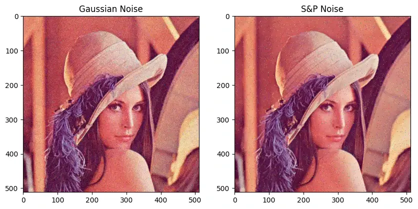
1 2 3 4 5 6 7 8 9 10 11 12 13 14 15 16 17 18 from skimage.util import random_noiseimg = cv2.imread("LenaRGB.bmp" ,1 ) img = cv2.cvtColor(img, cv2.COLOR_BGR2RGB) gaussian_noise = random_noise(img, mode='gaussian' , var=0.01 ) gaussian_noise = (gaussian_noise * 255 ).astype(np.uint8) sp_noise = random_noise(img, mode='s&p' , amount=0.02 ) sp_noise = (sp_noise * 255 ).astype(np.uint8) plt.figure(figsize=(10 , 5 )) plt.subplot(121 ) plt.imshow(gaussian_noise) plt.title("Gaussian Noise" ) plt.subplot(122 ) plt.imshow(sp_noise) plt.title("S&P Noise" )
通过各种滤波方式可以对噪声进行去除
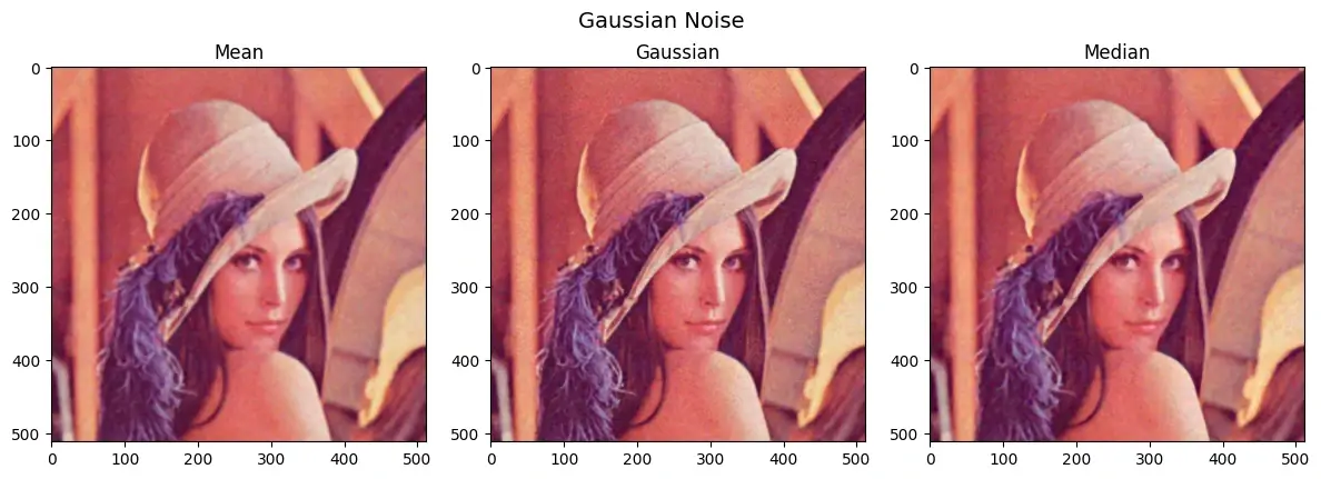
1 2 3 4 gauss_mean = cv2.blur(gaussian_noise, (5 , 5 )) gauss_gaussian = cv2.GaussianBlur(gaussian_noise, (5 , 5 ), 0 ) gauss_median = cv2.medianBlur(gaussian_noise, 5 )
均值滤波会平滑图像,使得图像稍微模糊一些,高斯滤波并不能完全去除高斯噪声
这是因为它只是一个低通滤波器,主要削弱高频分量,高斯噪声的高频部分会被削弱,但低频部分的噪声依然保留,所以它不能“专门去掉高斯噪声”,而只是做了一次模糊平均
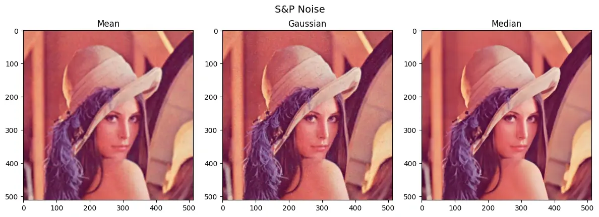
1 2 3 4 sp_mean = cv2.blur(sp_noise, (5 , 5 )) sp_gaussian = cv2.GaussianBlur(sp_noise, (5 , 5 ), 0 ) sp_median = cv2.medianBlur(sp_noise, 5 )
可以看到中值滤波对椒盐噪声的处理非常好,基本恢复原图的状态了
阈值分割 固定阈值分割 将灰度图像二值化或多阈值化,通过cv2.threshold()来实现阈值分割
1 cv2.threshold(img, thresh, maxval, type )
thresh: 阈值
maxval: 当像素值超过阈值时赋予的新值[用于THRESH_BINARY],一般为255
type:阈值类型(最重要)
阈值类型
高于阈值
低于阈值
应用
cv2.THRESH_BINARY(二值化)赋值为 maxval
赋值为 0
前景白、背景黑
cv2.THRESH_BINARY_INV(反二值化)赋值为 0
赋值为 maxval
背景白、前景黑
cv2.THRESH_TRUNC(截断)截断成阈值
保持原值
限制高光
cv2.THRESH_TOZERO保持原值
赋值为 0
滤掉低强度背景
cv2.THRESH_TOZERO_INV赋值为 0
保持原值
滤掉高亮区域
返回retval, dst
retval: 实际使用的阈值(在使用 THRESH_OTSU 或 THRESH_TRIANGLE 时特别有用)dst: 阈值化后的图像
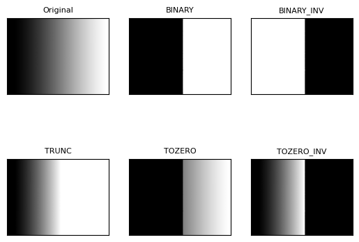
1 2 3 4 5 6 7 8 9 10 11 12 13 14 15 import matplotlib.pyplot as pltimg = cv2.imread("gradient_gray.png" , 0 ) _, dst1 = cv2.threshold(img,127 ,255 ,cv2.THRESH_BINARY) _, dst2 = cv2.threshold(img,127 ,255 ,cv2.THRESH_BINARY_INV) _, dst3 = cv2.threshold(img,127 ,255 ,cv2.THRESH_TRUNC) _, dst4 = cv2.threshold(img,127 ,255 ,cv2.THRESH_TOZERO) _, dst5 = cv2.threshold(img,127 ,255 ,cv2.THRESH_TOZERO_INV) titles = ['Original' , 'BINARY' , 'BINARY_INV' , 'TRUNC' , 'TOZERO' , 'TOZERO_INV' ] images = [img, dst1, dst2, dst3, dst4, dst5] for i in range (6 ): plt.subplot(2 , 3 , i + 1 ) plt.imshow(images[i], 'gray' ) plt.title(titles[i], fontsize=8 ) plt.xticks([]), plt.yticks([]) plt.show()
自适应阈值 cv2.adaptiveThreshold()自适应阈值会每次取图片的一小部分计算阈值,这样图片不同区域的阈值就不尽相同
1 thresholded_image = cv2.adaptiveThreshold(img, maxval, cv2.ADAPTIVE_THRESH_MEAN_C, cv2.THRESH_BINARY, block_size, C)
maxval:最大阈值,一般为 255
参数3:小区域阈值的计算方式
ADAPTIVE_THRESH_MEAN_C:小区域内取均值ADAPTIVE_THRESH_GAUSSIAN_C:小区域内加权求和,权重是个高斯核
参数4:阈值方法,只能使用THRESH_BINARY、THRESH_BINARY_INV
参数5:小区域的面积(正方形),输入边长(像素)
参数6:最终阈值等于小区域计算出的阈值再减去此值
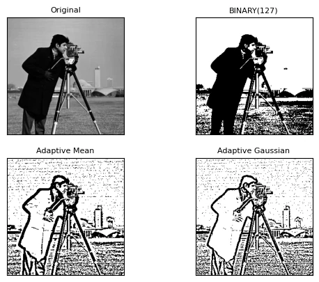
1 2 3 4 5 6 7 8 9 10 11 12 img = cv2.imread("Cameraman.bmp" , 0 ) _, dst1 = cv2.threshold(img,127 ,255 ,cv2.THRESH_BINARY) dst2 = cv2.adaptiveThreshold(img,255 ,cv2.ADAPTIVE_THRESH_MEAN_C,cv2.THRESH_BINARY,11 ,4 ) dst3 = cv2.adaptiveThreshold(img,255 ,cv2.ADAPTIVE_THRESH_GAUSSIAN_C, cv2.THRESH_BINARY,11 ,4 ) titles = ['Original' , 'BINARY(127)' , 'Adaptive Mean' , 'Adaptive Gaussian' ] images = [img, dst1, dst2, dst3] for i in range (4 ): plt.subplot(2 , 2 , i + 1 ) plt.imshow(images[i], 'gray' ) plt.title(titles[i], fontsize=8 ) plt.xticks([]), plt.yticks([]) plt.show()
Otsu’s阈值 在前面cv2.threshold() 用的是固定阈值,比如thresh=127
在很多场景下,图像亮度分布不均匀,固定阈值效果不好
Otsu’s方法是一种自适应阈值选择算法 ,通过分析图像灰度直方图,自动确定最佳分割阈值
核心思想是最大化前景(目标)与背景之间的类间方差
1 2 thresh_val, otsu_img = cv2.threshold(img, 0 , 255 , cv2.THRESH_BINARY + cv2.THRESH_OTSU)
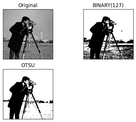
1 2 3 4 5 6 7 8 9 10 img = cv2.imread("Cameraman.bmp" , 0 ) _, dst1 = cv2.threshold(img , 127 , 255 , cv2.THRESH_BINARY) _, dst2 = cv2.threshold(img, 0 , 255 , cv2.THRESH_BINARY+cv2.THRESH_OTSU) imgs = [img, dst1, dst2] titles = ["Original" , "BINARY(127)" , "OTSU" ] for i in range (3 ): plt.subplot(2 , 2 , i + 1 ) plt.imshow(imgs[i], cmap='gray' ) plt.title(titles[i]) plt.xticks([]), plt.yticks([])
边缘检测 图像边缘检测是计算机视觉和图像处理中的一项基本任务,它用于识别图像中亮度变化明显的区域,这些区域通常对应于物体的边界
边缘检测通常基于梯度 (Gradient),它表示图像强度变化的方向和大小
一维情况下:边缘 = 信号一阶导数极大值位置
二维情况下
常用的梯度算子如下:
算法
核心
适用场景
缺点
Sobel算子
一阶导数(差分)+平滑
检测水平和垂直边缘
边缘定位精度一般,特别是对斜向边缘不够准确
Scharr算子
优化的Sobel
检测细微的边缘
计算量略高于Sobel,低分辨率图片差别不大
Laplacian算子
二阶导数
检测边缘和角点
对噪声非常敏感,检测结果往往是“双边缘”
数值转化 常见算子通常用 CV_64F 或 CV_32F 保存结果,计算出来的结果是float类型,包含负数
OpenCV的imshow和Matplotlib的imshow(cmap="gray") 都假定数据范围在[0,255](或 [0,1]浮点)
如果直接显示float图像,会导致数据被自动线性拉伸,结果和实际数值分布不符
如果为了清晰判断与分析边缘,需要对其进行cv2.convertScaleAbs()处理,这样能保证边缘效果直观可见
如果后续还需要进行一些运算,就不能取cv2.convertScaleAbs(),因为符号信息在一些算法里是有意义的,此时保留float 原始结果更合理
1 magnitude = cv2.magnitude(sobelx, sobely)
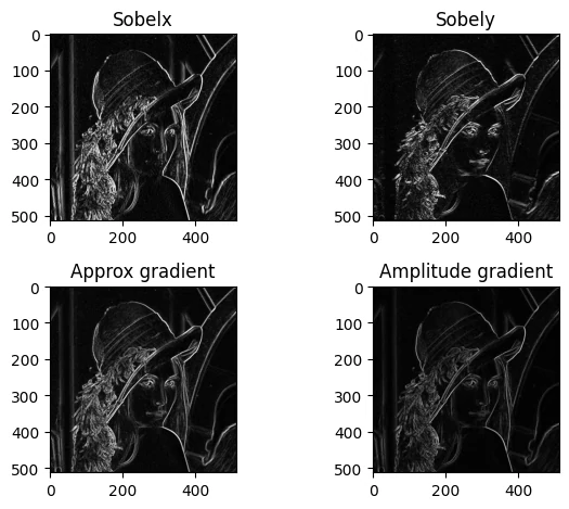
Sobel算子 Sobel算子是一种基于梯度的边缘检测算子,它通过计算图像在水平和垂直方向上的梯度来检测边缘,结合了高斯平滑和微分操作,因此对噪声具有一定的抑制作用
水平方向卷积核 [[-1, 0, 1], [-2, 0, 2], [-1, 0, 1]]
垂直方向卷积核 [[-1, -2, -1], [0, 0, 0], [1, 2, 1]]
1 2 3 4 5 6 7 8 9 10 11 12 13 14 15 16 17 18 19 20 21 22 23 24 25 img = cv2.imread("Lena.bmp" , 0 ) sobelx = cv2.Sobel(img, cv2.CV_64F, 1 , 0 , ksize=3 ) sobely = cv2.Sobel(img, cv2.CV_64F, 0 , 1 , ksize=3 ) sobelx_abs = cv2.convertScaleAbs(sobelx) sobely_abs = cv2.convertScaleAbs(sobely) grad = cv2.addWeighted(sobelx_abs, 0.5 , sobely_abs, 0.5 , 0 ) sobel = cv2.magnitude(sobelx, sobely) plt.subplot(221 ) plt.imshow(sobelx_abs, cmap='gray' ) plt.title('Sobelx' ) plt.subplot(222 ) plt.imshow(sobely, cmap='gray' ) plt.title('Sobely' ) plt.subplot(223 ) plt.imshow(grad, cmap='gray' ) plt.title('Approx gradient' ) plt.subplot(224 ) plt.imshow(sobel_abs, cmap='gray' ) plt.title('Amplitude gradient' ) plt.tight_layout()
Scharr算子 是Sobel的改进版,权重更大,在小核(3×3)时效果优于 Sobel
水平方向卷积核 [[-3, 0, 3], [-10, 0, 10], [-3, 0, 3]]
垂直方向卷积核 [[-3, -10, -3], [0, 0, 0], [3, 10, 3]]
1 2 scharrx = cv2.Scharr(img, cv2.CV_64F, 1 , 0 ) scharry = cv2.Scharr(img, cv2.CV_64F, 0 , 1 )
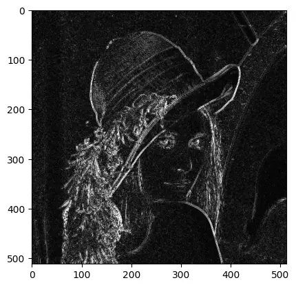
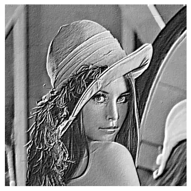
Laplacian算子 Laplacian算子是一种二阶微分算子,它通过计算图像的二阶导数来检测边缘,但对噪声比较敏感,因此通常在使用之前会对图像进行高斯平滑处理
卷积核 [[0, 1, 0], [1, -4, 1], [0, 1, 0]]
1 laplacian = cv2.Laplacian(img, cv2.CV_64F, ksize=1 , scale=1 , borderType=cv2.BORDER_DEFAULT)
ksize:Laplacian核的大小,默认为 1
并不是代表卷积核大小为1,而是最基本的二阶差分算子
scale:缩放因子,默认为 1
1 2 3 4 img = cv2.imread("Lena.bmp" , 0 ) laplacian = cv2.Laplacian(img, cv2.CV_64F,ksize=3 ) laplacian_abs = cv2.convertScaleAbs(laplacian) plt.imshow(laplacian_abs, cmap='gray' )
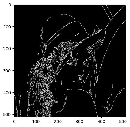
Canny边缘检测🔥 稳定、精确,最常用
由John F. Canny提出,主要包括以下几个步骤:
噪声抑制:使用高斯滤波器对图像进行平滑处理,以减少噪声的影响
计算梯度:使用Sobel算子计算图像的梯度幅值和方向
非极大值抑制(NMS):沿着梯度方向,保留局部梯度最大的像素点,删除不被认为是边缘一部分的像素,只有细线候选边缘将保留
双阈值检测:使用两个阈值(低阈值和高阈值)来确定真正的边缘
如果像素梯度高于高阈值,则该像素被接受为边缘
如果像素梯度值低于下限阈值,则将其拒绝
如果像素梯度介于两个阈值之间,则只有当它连接到高于上限阈值的像素时,才会被接受
1 edges = cv2.Canny(img, threshold1, threshold2, apertureSize=3 , L2gradient=False )
img:必须是单通道的灰度图像
threshold1:低阈值越低,检测到的候选点越多,但噪声也会增多
threshold2:高阈值越高,检测到的边缘越少,但更可靠,高阈值通常是低阈值的2-3倍
apertureSize:Sobel算子的孔径大小,默认为3
L2gradient:是否使用 L2 范数计算梯度幅值,默认为 False
1 2 3 img = cv2.imread("LEna.bmp" , 0 ) edges = cv2.Canny(img, 100 , 200 ) plt.imshow(edges, cmap='gray' )
创建滑动条 1 2 3 4 5 6 7 8 9 10 11 12 13 14 15 16 17 18 def nothing (x ): pass img = cv2.imread("Lena.bmp" , 0 ) plt.imshow(img, cmap='gray' ) cv2.namedWindow("Canny Edge Detection" ) cv2.createTrackbar("threshold1" ,"Canny Edge Detection" , 0 , 255 , nothing) cv2.createTrackbar("threshold2" ,"Canny Edge Detection" , 0 , 255 , nothing) while True : threshold1 = cv2.getTrackbarPos("threshold1" , "Canny Edge Detection" ) threshold2 = cv2.getTrackbarPos("threshold2" , "Canny Edge Detection" ) edges = cv2.Canny(img, threshold1, threshold2) cv2.imshow("Canny Edge Detection" , edges) if cv2.waitKey(0 ) & 0xFF == 27 : break cv2.destroyAllWindows()
自适应阈值设置 1 2 3 4 5 6 7 8 9 10 11 12 13 14 15 def auto_canny (img, sigma=0.33 ): v = np.median(img) lower = int (max (0 , (1.0 - sigma) * v)) upper = int (min (255 , (1.0 + sigma) * v)) edges = cv2.Canny(img, lower, upper) return edges, lower, upper img = cv2.imread("Lena.bmp" , 0 ) adaptive_edges, lower, upper = auto_canny(img) plt.imshow(adaptive_edges, cmap='gray' ) print (f"threshold1: {lower} , threshold2: {upper} " )
Otsu计算最佳阈值 1 2 3 4 5 6 7 8 9 10 11 12 13 14 15 def otsu_canny (img ): otsu_thresh, _ = cv2.threshold(img, 0 , 255 , cv2.THRESH_BINARY + cv2.THRESH_OTSU) lower = int (otsu_thresh * 0.5 ) upper = int (otsu_thresh) edges = cv2.Canny(img, lower, upper) return edges, lower, upper img = cv2.imread("Lena.bmp" , 0 ) otsu_edges, lower, upper = otsu_canny(img) plt.imshow(otsu_edges, cmap='gray' ) print (f"threshold1: {lower} , threshold2: {upper} " )
实时边缘检测 结合滑动条,控制Canny的两个阈值,视频部分后面章节具体讲
1 2 3 4 5 6 7 8 9 10 11 12 13 14 15 16 17 18 19 20 21 22 23 24 25 26 27 28 def nothing (x ): pass cv2.namedWindow("Overlay" ) cv2.createTrackbar("threshold1" ,"Overlay" , 0 , 255 , nothing) cv2.createTrackbar("threshold2" ,"Overlay" , 0 , 255 , nothing) cap = cv2.VideoCapture("camera_vedio.mp4" ) while True : ret, frame = cap.read() threshold1 = cv2.getTrackbarPos("threshold1" , "Overlay" ) threshold2 = cv2.getTrackbarPos("threshold2" , "Overlay" ) if not ret: cap.set (cv2.CAP_PROP_POS_FRAMES, 0 ) continue gray = cv2.cvtColor(frame,cv2.COLOR_BGR2GRAY) edges = cv2.Canny(gray, threshold1, threshold2) edges_color = cv2.cvtColor(edges, cv2.COLOR_GRAY2BGR) overlay = cv2.addWeighted(frame, 0.8 , edges_color, 0.5 , 0 ) cv2.imshow("Overlay" , overlay) if cv2.waitKey(30 ) & 0xFF == 27 : break cap.release() cv2.destroyAllWindows()
或者也可以利用edges实现掩膜上色
1 2 3 4 5 6 7 8 9 10 11 12 13 14 cap = cv2.VideoCapture("camera_vedio.mp4" ) while True : ret, frame = cap.read() if not ret: break gray = cv2.cvtColor(frame,cv2.COLOR_BGR2GRAY) edges = cv2.Canny(gray, 100 , 200 ) mask = edges > 0 frame[mask] = [0 ,0 ,255 ] cv2.imshow("Edges on Original" , frame) if cv2.waitKey(30 ) & 0xFF == ord ('q' ): break cap.release() cv2.destroyAllWindows()
形态变换 形态学变换是一些基于图像形状的简单操作,它通常在二值图像上执行
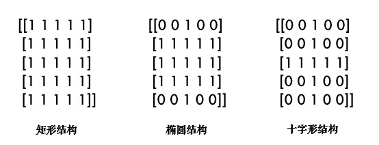
它需要两个输入,一个是原始图像,第二个称为结构元素或内核,它决定操作的性质
两种基本的形态学算子是腐蚀和膨胀
操作 函数 应用场景
腐蚀 cv2.erode()去除噪声、分离物体
膨胀 cv2.dilate()连接断裂的物体、填充空洞
开运算 cv2.morphologyEx()去除小物体、平滑物体边界
闭运算 cv2.morphologyEx()填充小孔洞、连接邻近物体
形态学梯度 cv2.morphologyEx()提取物体边缘
腐蚀 腐蚀操作是一种缩小图像中前景对象的过程,其原理是在原图的小区域内取局部最小值,小区域内有一个是0该像素点就为0(用numpy实现就是遍历选一个region取其中min)
1 cv2.erode(img, kernel, iterations=1 )
1 2 3 4 img = cv2.imread("imgs/j.png" ,0 ) kernel = cv2.getStructuringElement(cv2.MORPH_RECT, (5 , 5 )) erosion = cv2.erode(img, kernel, iterations=1 ) plt.imshow(erosion,cmap="gray" )
膨胀 膨胀操作与腐蚀相反,它是一种扩大图像中前景对象的过程
1 cv2.dilate(src, kernel, iterations=1 )
1 2 3 img = cv2.imread("imgs/j.png" ,0 ) dilate = cv2.dilate(img, kernel, iterations=1 ) plt.imshow(dilate,cmap="gray" )
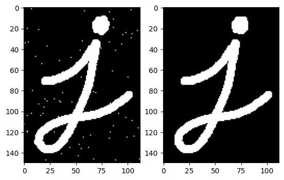
开运算 开运算只是先腐蚀后膨胀 的另一种说法,用于去除小的白色噪声点
cv2.MORPH_OPEN
1 2 3 4 5 6 7 8 9 10 11 12 13 14 15 16 from skimage.util import random_noiseimg = cv2.imread("imgs/j.png" ,0 ) noise_full = random_noise(np.zeros_like(img), mode='s&p' , amount=0.01 ) noise_full = (noise_full * 255 ).astype(np.uint8) mask = (img == 0 ) sp_noise = img.copy() sp_noise[mask] = noise_full[mask] open = cv2.morphologyEx(sp_noise, cv2.MORPH_OPEN, kernel)plt.subplot(121 ) plt.imshow(sp_noise, cmap="gray" ) plt.subplot(122 ) plt.imshow(open ,cmap="gray" )
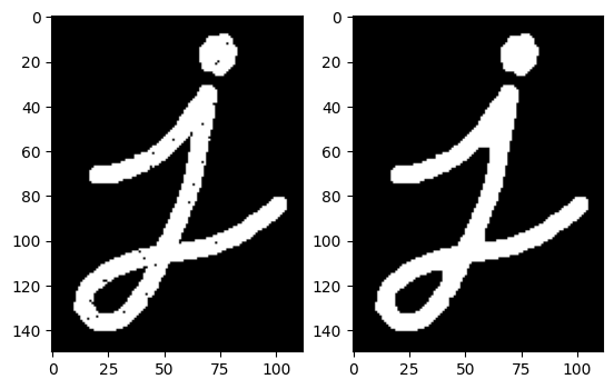
闭运算 闭运算是开运算的逆运算,先膨胀后腐蚀 ,用于填充白色区域内部的小黑洞
cv2.MORPH_CLOSE
1 2 3 4 5 6 7 8 9 10 11 12 13 14 15 16 17 from skimage.util import random_noiseimg = cv2.imread("imgs/j.png" ,0 ) white_bg = np.ones_like(img, dtype=np.float32) noise_full = random_noise(white_bg, mode='s&p' , amount=0.01 ) noise_full = (noise_full * 255 ).astype(np.uint8) mask = (img == 255 ) sp_noise = img.copy() sp_noise[mask] = noise_full[mask] close = cv2.morphologyEx(sp_noise, cv2.MORPH_CLOSE, kernel) plt.subplot(121 ) plt.imshow(sp_noise, cmap="gray" ) plt.subplot(122 ) plt.imshow(close,cmap="gray" )
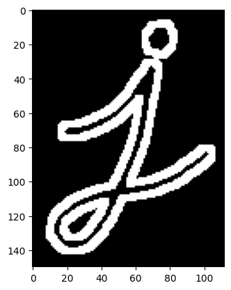
形态学梯度 形态学梯度是膨胀图像与腐蚀图像的差值,主要用于提取图像中前景对象的边缘
cv2.MORPH_GRADIENT
1 2 3 img = cv2.imread("imgs/j.png" ,0 ) gradient = cv2.morphologyEx(img, cv2.MORPH_GRADIENT, kernel) plt.imshow(gradient, cmap="gray" )
小总结 一般常见的图像处理流程:
读取+灰度化:减少计算量,很多算子只需要单通道;特殊情况保持彩色(比如分割 RGB/HSV特征)
降噪(平滑):均值滤波/高斯滤波/中值滤波,让后续边缘检测或分割更稳定
增强(对比度提升,锐化):直方图均衡化/CLAHE → 提升对比度;卷积或Unsharp Mask → 突出细节;[会造成噪声加剧 ]
阈值分割:固定阈值、Otsu、自适应阈值,得到前景/背景的mask
边缘检测:Canny(最主要),可直接基于分割结果做轮廓提取
方法
结果特点
适用场景
灰度图做边缘检测
包含更多细节(比如纹理),但噪声多
需要提取细微边缘(如纹理、阴影)
阈值图做边缘检测
轮廓更简洁(闭合),噪声少
需要提取物体轮廓(如零件、数字)
形态学处理:膨胀/腐蚀:强化结构特征;形态学梯度:得到轮廓;开/闭运算:去小噪点/填小孔洞[针对的是二值图 ,无论阈值分割还是边缘检测得到的结果都是二值图]
这些步骤并不是固定且必须的
图像增强 :读取 → 灰度化 → 去噪/平滑 → 对比度/亮度增强 → 锐化
图像恢复 :读取 → 灰度化 → 退化模型估计 → 去噪/去模糊 → 恢复图像
图像分割 :读取 → 灰度化 → 阈值分割或边缘检测 → 形态学处理 → 区域标记
特征提取 :读取 → 灰度化 → 平滑 → 边缘/角点检测 → 特征提取
图像轮廓 轮廓可以简单地解释为连接所有连续点(沿边界)的曲线,这些点具有相同的颜色或强度
轮廓和边缘很像,不过轮廓是连续的,边缘并不全都连续
轮廓是用于形状分析和对象检测与识别的有用工具
为了获得更高的精度,需要使用二值图像
寻找轮廓是针对白色物体的,一定要保证物体是白色,而背景是黑色
主要流程及函数:
步骤 函数
图像预处理(转灰度)
cv2.cvtColor()
二值化处理
cv2.threshold()
查找轮廓
cv2.findContours()
绘制轮廓
cv2.drawContours()
计算轮廓面积
cv2.contourArea()
计算轮廓周长
cv2.arcLength()
计算边界矩形
cv2.boundingRect()
计算最小外接矩形
cv2.minAreaRect()
计算最小外接圆
cv2.minEnclosingCircle()
多边形逼近
cv2.approxPolyDP()
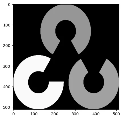
代码框架:
1 2 3 4 5 img = cv2.imread("imgs/match_shape.jpg" ,1 ) gray = cv2.cvtColor(img, cv2.COLOR_BGR2GRAY) _, thresh = cv2.threshold(gray, 0 , 255 , cv2.THRESH_BINARY+cv2.THRESH_OTSU) contours, hierarchy = cv2.findContours(thresh, 3 , 2 ) cv2.drawContours(img, contours, -1 , (0 ,255 ,0 ),2 )
寻找轮廓 cv2.findContours()用于在二值图像中查找轮廓
1 2 3 4 5 contours, hierarchy = cv2.findContours( image, mode, method )
mode: 轮廓检索模式,常用的有:
cv2.RETR_EXTERNAL/1: 只检测最外层轮廓cv2.RETR_LIST/2: 检测所有轮廓,但不建立层次关系cv2.RETR_TREE/3: 检测所有轮廓,并建立完整的层次结构(常用)cv2.RETR_CCOMP:把所有的轮廓只分为2个层级,不是外层的就是里层的
method: 轮廓近似方法,常用的有:
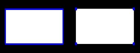
cv2.CHAIN_APPROX_NONE/1: 存储所有的轮廓点,轮廓很密
cv2.CHAIN_APPROX_SIMPLE/2: 压缩水平、垂直和对角线段,只保留端点(常用)
第一张图像显示使用cv.CHAIN_APPROX_NONE获得的点(734)
第二张图像显示了使用cv.CHAIN_APPROX_SIMPLE获得的点(4)
返回值 :
contours: 检测到的轮廓列表,以数组形式存储,记录了每条轮廓的所有像素点的坐标hierarchy: 轮廓的层次结构信息
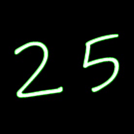
1 2 3 4 img = cv2.imread("imgs/2&5.png" ,1 ) gray = cv2.cvtColor(img, cv2.COLOR_BGR2GRAY) _, binary = cv2.threshold(gray, 0 , 255 , cv2.THRESH_BINARY+cv2.THRESH_OTSU) contours, hierarchy = cv2.findContours(binary, cv2.RETR_TREE, cv2.CHAIN_APPROX_SIMPLE)
绘制轮廓 cv2.drawContours()用于在图像上绘制检测到的轮廓
1 cv2.drawContours(img, contours, contourIdx, color, thickness)
contours: 轮廓列表contourIdx: 要绘制的轮廓索引,如果为负数,则绘制所有轮廓thickness:线宽,设为-1时将填充轮廓
无返回值,直接在输入图像上绘制轮廓
1 2 cv2.drawContours(img, contours, -1 , (0 ,255 ,0 )) cv2.drawContours(img, contours, 3 , (0 ,255 ,0 ))
但很多情况下,会以以下方式绘制单个轮廓
1 2 cnt = contours[3 ] cv2.drawContours(img, [cnt], 0 , (0 ,255 ,0 ))
1 2 3 4 cv2.drawContours(img, contours, -1 , (0 ,255 ,0 ),2 ) cv2.imshow("Contours" , img) cv2.waitKey(0 ) cv2.destroyAllWindows()
轮廓特征 轮廓属性 :
1 2 cnt = contours[0 ] M = cv2.moments(cnt)
图像矩可以帮助计算一些特征,例如轮廓的质心:
1 2 3 cx = int (M['m10' ]/M['m00' ]) cy = int (M['m01' ]/M['m00' ]) print (cx,cy)
轮廓的面积:
1 2 area = cv2.contourArea(cnt) area = M['m00' ]
计算轮廓的周长或弧长:
1 length = cv2.arcLength(cnt, True )
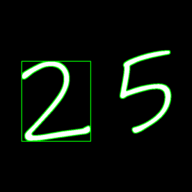
边界矩形 1 2 x, y, w, h = cv2.boundingRect(cnt) cv2.rectangle(img,(x,y),(x+w,y+h),(0 ,255 ,0 ),2 )
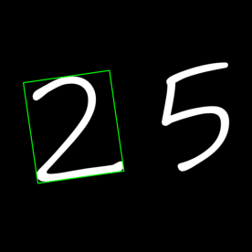
最小外接矩形 1 2 3 4 rect = cv2.minAreaRect(cnt) box = cv2.boxPoints(rect) box = box.astype(int ) cv2.drawContours(img, [box], -1 , (0 , 255 , 0 ),2 )
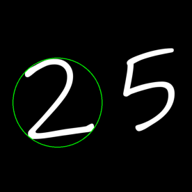
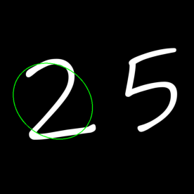
最小外接圆 1 2 3 4 (x,y), radius = cv2.minEnclosingCircle(cnt) center = (int (x),int (y)) radius = int (radius) cv2.circle(img,center,radius,(0 ,255 ,0 ),2 )
椭圆拟合 1 2 3 img = cv2.imread("imgs/2&5.png" ,1 ) ellipse = cv2.fitEllipse(cnt) cv2.ellipse(img,ellipse,(0 ,255 ,0 ),2 )
多边形逼近 根据指定的精度将轮廓形状逼近到具有较少顶点的另一个形状,这是Douglas-Peucker算法 的一种实现
1 approx = cv2.approxPolyDP(cnt, epsilon, True )
epsilon:轮廓到逼近轮廓的最大距离,值越小,近似越精确
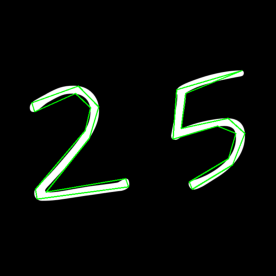
1 2 3 4 5 img = cv2.imread("imgs/2&5.png" ,1 ) for contour in contours: epsilon = 0.01 *cv2.arcLength(contour,True ) approx = cv2.approxPolyDP(contour,epsilon,True ) cv2.drawContours(img,[approx],0 ,(0 ,255 ,0 ),2 )
凸包 在二维平面里,给定一组点,凸包就是能把这些点“包”起来的最小凸多边形
凸包看起来类似于轮廓逼近,但并非如此(在某些情况下,两者可能提供相同的结果)
凸包的边界都是凸的,没有凹进去的部分
OpenCV 提供了 cv2.convexHull 来计算凸包
1 hull = cv2.convexHull(points[, hull[, clockwise[, returnPoints]]])
points:输入点集(通常是 contour)
hull:输出索引,通常避免使用它
clockwise:方向标志,True 表示顺时针,False 表示逆时针
returnPoints:True(默认):返回点坐标;False:返回的是点的索引
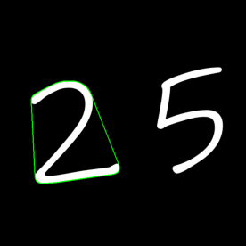
1 2 3 img = cv2.imread("imgs/2&5.png" ,1 ) hull = cv2.convexHull(cnt) cv2.drawContours(img,[hull],0 ,(0 ,255 ,0 ),2 )
如果想查找凸性缺陷,则需要将 returnPoints 设置为 False
1 2 3 4 5 6 7 8 9 10 11 12 13 14 [[[390 289 ]] [[395 290 ]] [[399 291 ]] ...] [[521 ] [519 ] [517 ] ...] print (cnt[hull[:3 ]])[[[[390 289 ]]] [[[395 290 ]]] [[[399 291 ]]]]
可以通过cv.isContourConvex()判断曲线是否为凸
1 is_convex = cv2.isContourConvex(cnt)
轮廓属性 长宽比 :边界矩形的宽高比
1 2 x,y,w,h = cv.boundingRect(cnt) aspect_ratio = w/h
范围 :轮廓面积与边界矩形面积的比值
1 2 3 4 area = cv.contourArea(cnt) x,y,w,h = cv.boundingRect(cnt) rect_area = w*h extent = area/rect_area
实体度 :轮廓面积与其凸包面积的比值
1 2 3 hull = cv2.convexHull(cnt) hull_area = cv2.contourArea(hull) solidity = area/hull_area
等效直径 :与轮廓面积相同的圆的直径
1 equi_diameter = np.sqrt(4 *area/np.pi)
掩模
1 2 3 4 5 mask = np.zeros(gray.shape,np.uint8) cv2.drawContours(mask,[cnt],0 ,255 ,-1 ) pixelpoints = np.transpose(np.nonzero(mask))
Numpy以**(行,列)格式给出坐标,而OpenCV以 (x,y)**格式给出坐标
获得掩膜以后可以利用它进行一些计算
最大值、最小值及其位置:
1 min_val, max_val, min_loc, max_loc = cv.minMaxLoc(gray, mask = mask)
平均颜色或平均强度:
1 mean_val = cv.mean(img, mask = mask)
极值点 :
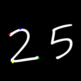
极值点是指对象的最高点、最低点、最右点和最左点
1 2 3 4 5 6 7 8 9 10 leftmost = tuple (cnt[cnt[:,:,0 ].argmin()][0 ]) rightmost = tuple (cnt[cnt[:,:,0 ].argmax()][0 ]) topmost = tuple (cnt[cnt[:,:,1 ].argmin()][0 ]) bottommost = tuple (cnt[cnt[:,:,1 ].argmax()][0 ]) cv2.circle(img, leftmost, 8 , (0 ,0 ,255 ), -1 ) cv2.circle(img, rightmost, 8 , (0 ,255 ,0 ), -1 ) cv2.circle(img, topmost, 8 , (255 ,0 ,0 ), -1 ) cv2.circle(img, bottommost, 8 , (0 ,255 ,255 ), -1 ) plt.imshow(cv2.cvtColor(img, cv2.COLOR_BGR2RGB))
简单案例(数硬币) 写一个函数,统计图像中“物体的数量和面积分布”(比如数硬币)
1 2 3 4 5 6 7 8 9 10 11 12 13 14 15 16 17 18 19 20 21 22 23 24 25 26 27 28 29 30 31 32 33 34 35 36 37 38 39 40 41 import cv2import numpy as npdef count_objects (img_path, show = False , min_area=100 ): img = cv2.imread(img_path) gray = cv2.cvtColor(img, cv2.COLOR_BGR2GRAY) _ , thresh = cv2.threshold(gray, 20 , 255 , cv2.THRESH_BINARY) kernel = cv2.getStructuringElement(cv2.MORPH_ELLIPSE, (7 , 7 )) open = cv2.morphologyEx(thresh, cv2.MORPH_OPEN,kernel) contours, _ = cv2.findContours(open , 3 , 2 ) areas = [] valid_contours = [] for cnt in contours: area = cv2.contourArea(cnt) if area >= min_area: areas.append(area) valid_contours.append(cnt) object_num = len (valid_contours) if show: cv2.drawContours(img, valid_contours, -1 , (0 , 255 , 0 )) cv2.imshow('Objects' , img) contour_img = np.zeros_like(img) cv2.drawContours(contour_img, contours, -1 , (0 , 255 , 0 )) cv2.imshow('Contours' , contour_img) cv2.waitKey(0 ) cv2.destroyAllWindows() return object_num, areas if __name__ == '__main__' : object_num, areas = count_objects('imgs/coins.webp' ,True ) print (f"The num of coins: {object_num} " ) print (f"The area of each coin: {areas} " )
形状匹配 cv2.matchShapes()可以检测两个形状之间的相似度,返回值越小,越相似
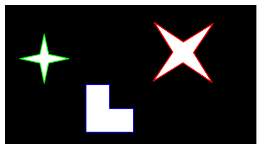
1 2 3 4 5 6 7 8 9 10 11 12 13 img = cv2.imread("imgs/match_shape.jpg" ,1 ) gray = cv2.cvtColor(img, cv2.COLOR_BGR2GRAY) _, thresh = cv2.threshold(gray, 0 , 255 , cv2.THRESH_BINARY+cv2.THRESH_OTSU) contours, hierarchy = cv2.findContours(thresh, 3 , 2 ) cnt_a, cnt_b, cnt_c = contours[0 ], contours[1 ], contours[2 ] cv2.drawContours(img, [cnt_a], 0 , (255 , 0 , 0 ), 2 ) cv2.drawContours(img, [cnt_b], 0 , (0 , 255 , 0 ), 2 ) cv2.drawContours(img, [cnt_c], 0 , (0 , 0 , 255 ), 2 ) plt.imshow(cv2.cvtColor(img, cv2.COLOR_BGR2RGB)) plt.axis("off" ) print (cv2.matchShapes(cnt_a, cnt_b, 1 , 0.0 )) print (cv2.matchShapes(cnt_a, cnt_c, 1 , 0.0 )) print (cv2.matchShapes(cnt_b, cnt_c, 1 , 0.0 ))
bc的输出最低,根据颜色,bc对应绿色和红色,符合预期
直方图 在图像处理中,直方图是一种非常重要的工具,它可以帮助我们了解图像的像素分布情况
三个主要概念:
BIN(区间) : 如果统计0~255每个像素值,BIN=256;如果划分区间,比如0~15,16~31...,那么BIN=16,BIN在OpenCV文档中由histSize表示
DIMS(维度) : 要计算的通道数,对于灰度图为1,普通彩色图为3
RANGE(范围) : 要计算的像素值范围,一般为[0,256],即所有强度值
计算直方图 使用 cv2.calcHist() 函数来计算图像的直方图
1 cv2.calcHist(imgs, channels, mask, histSize, ranges)
imgs: 输入的图像列表,通常是一个包含单通道或多通道图像的列表,通常输入[img]
channels:需要计算直方图的通道索引,灰度图像为[0],彩色图像选择[0/1/2]|(BGR)
mask: 掩膜,指定掩膜后只计算掩膜内的像素,如果没有输入None
可以用阈值分割后的二值图也可以自己创建,比如
1 2 mask = np.zeros(img.shape[:2 ], np.uint8) mask[100 :300 , 100 :300 ] = 255
histSize:直方图的BIN数量,灰度图像通常输入[256]
ranges: 像素值的范围,对于灰度图像,通常设置为[0, 256]
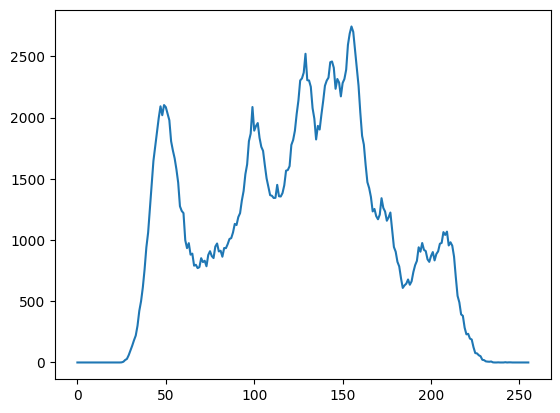
灰度:
1 2 3 img = cv2.imread("imgs/Lena.bmp" , 0 ) hist = cv2.calcHist([img],[0 ],None ,[256 ],[0 ,256 ]) plt.plot(hist)
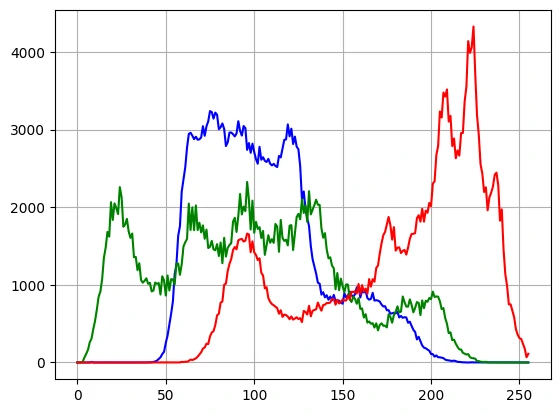
彩色:
1 2 3 4 5 img = cv2.imread("imgs/LenaRGB.bmp" , 1 ) colors = ('b' , 'g' , 'r' ) for i, colors in enumerate (colors): hist = cv2.calcHist([img],[i],None ,[256 ],[0 ,256 ]) plt.plot(hist, color = colors)
Numpy还提供了一个函数np.histogram(),在这里还要将将多维数组展平(np.ravel())
1 hist,bins = np.histogram(img.ravel(),256 ,[0 ,256 ])
还有一种针对灰度图的更高效方式:
1 hist = np.bincount(img.ravel(), minlength=256 )
但其实还是cv2的性能高
绘制直方图 刚刚直接用的plot将数据以曲线的形式绘制出来,但这并不是常见直方图的模样
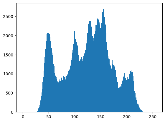
Matplotlib 带有一个直方图绘图函数:matplotlib.pyplot.hist()
可以直接输入图像,不需要先cv2.calcHist()
1 2 img = cv2.imread("imgs/Lena.bmp" , 0 ) plt.hist(img.ravel(), 256 , [0 , 256 ])
但对于彩色图样,选择普通绘图反而是更好的选择,因为这样可以很容易看出不同颜色的成分
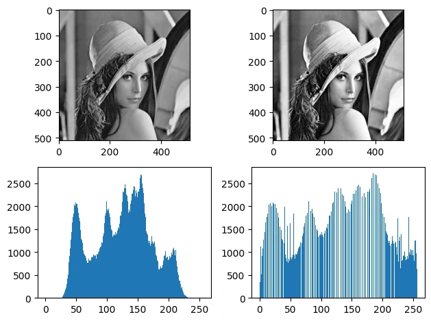
直方图均衡化 直方图均衡化是一种增强图像对比度的方法,通过重新分配像素强度值,使直方图更加均匀,改善图像的全局亮度和对比度
1 eq_img = cv2.equalizeHist(img)
1 2 3 4 5 6 7 8 9 10 11 12 img = cv2.imread("imgs/Lena.bmp" , 0 ) eq_img = cv2.equalizeHist(img) plt.subplot(221 ) plt.imshow(img,'gray' ) plt.subplot(222 ) plt.imshow(eq_img,'gray' ) plt.subplot(223 ) plt.hist(img.ravel(), 256 , [0 , 256 ]) plt.subplot(224 ) plt.hist(eq_img.ravel(), 256 , [0 , 256 ]) plt.tight_layout() plt.show()
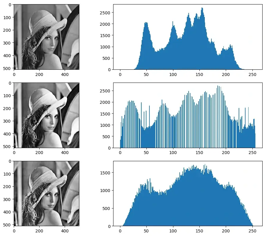
自适应均衡化 直方图均衡化是应用于整幅图片的,但是这可能导致局部细节丢失,自适应均衡化就是用来解决这一问题的,它在每一个小区域内(默认 8×8)进行直方图均衡化
当然,如果有噪声的话也会被放大,所以需要对对比度进行限制,所以这个算法全称叫对比度受限的自适应直方图均衡化CLAHE
1 clahe = cv2.createCLAHE(clipLimit=2.0 , tileGridSize=(8 , 8 ))
可以看到不会有过曝区域
直方图比较 cv2.compareHist() 函数,用于比较两个直方图的相似度
1 similarity = cv2.compareHist(hist1, hist2, method)
比较方法主要有四种:
方法
代码标识
范围
相似性判断
衡量目标
相关性
cv2.HISTCMP_CORREL|0[-1,1]
越大越相似
直方图形状相似性
卡方
cv2.HISTCMP_CHISQR|1[0,+∞]
越小越相似
概率分布差异
相交
cv2.HISTCMP_INTERSECT|2[0,sum]
越大越相似
重叠部分
巴氏距离
cv2.HISTCMP_BHATTACHARYYA|3[0,1]
越小越相似
概率分布相似性
举例,直方图A = [1, 2, 3],直方图 B = [3, 2, 1]
Correlation: -0.999999999999998 (负相关)
方法
常见场景
相关性
检测线性相关性(亮度/对比度变化),找风格相似的图片
卡方
目标识别时发现差异
相交
直方图快速匹配
巴氏距离
目标跟踪,适合高精度相似性度量
在进行比较之前,一般都要进行归一化
使用cv2.normalize()
1 cv2.normalize(src, dst=None , alpha=1 , beta=0 , norm_type)
归一化常见方式:
函数
目的
常见用途
cv2.NORM_MINMAX把数据线性拉伸到[alpha, beta]区间
图像对比度拉伸
cv2.NORM_L1|2所有值除以绝对值和
直方图归一化为概率分布
cv2.NORM_L2(默认)|4所有值除以平方和的平方根
把向量长度归一到 1
匹配比较方法和归一化方式
方法
归一化方式
原因
相关性
无需
相关性看趋势,线性缩放不影响结果
卡方
L1
通常用于比较概率分布,需要归一化到概率分布
交集
不归一化/L1
不归一化为绝对重叠数量;
巴氏距离
L1
定义基于概率分布,需要归一化到概率分布
对于直方图均衡化后的图片,这四个方法其实都不太能看出是一张图
1 2 3 4 5 6 7 8 9 10 11 12 13 14 15 16 17 18 19 20 img = cv2.imread("imgs/Lena.bmp" , 0 ) eq_img = cv2.equalizeHist(img) hist_img = cv2.calcHist([img], [0 ], None , [256 ], [0 , 256 ]) cv2.normalize(hist_img, hist_img, alpha=1 , beta=0 , norm_type=cv2.NORM_L1) hist_eq = cv2.calcHist([eq_img], [0 ], None , [256 ], [0 , 256 ]) cv2.normalize(hist_eq, hist_eq, alpha=1 , beta=0 , norm_type=cv2.NORM_L1) methods = { "Correlation" : cv2.HISTCMP_CORREL, "Chi-Square" : cv2.HISTCMP_CHISQR, "Intersection" : cv2.HISTCMP_INTERSECT, "Bhattacharyya" : cv2.HISTCMP_BHATTACHARYYA } for name, method in methods.items(): score = cv2.compareHist(hist_img, hist_eq, method) print (f"{name} : {score} " )
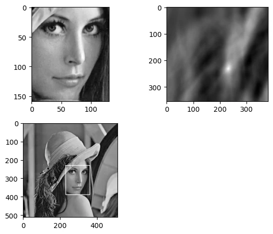
模板匹配 模板匹配是一种在较大的图像中搜索和查找模板图像位置的方法
用cv2.matchTemplate()实现模板匹配,返回的是一副灰度图,最白的地方表示最大的匹配
1 cv2.matchTemplate(img, templ, method)
method:匹配方法,有几种不同的计算方式
cv2.TM_CCOEFF / cv2.TM_CCOEFF_NORMED (相关系数,常用,越大越像)
cv2.TM_CCORR / cv2.TM_CCORR_NORMED (相关匹配,越大越像,效果不好,用的少)
cv2.TM_SQDIFF / cv2.TM_SQDIFF_NORMED (平方差,数值越小越像)
使用cv2.minMaxLoc()函数可以得到匹配值极值的坐标,以这个点为左上角角点,模板的宽和高画矩形就是匹配的位置了
1 min_val, max_val, min_loc, max_loc = cv2.minMaxLoc(result)
如果用的是平方差类方法TM_SQDIFF,数值越小越好,所以取min_loc,其他方法数值越大越好,所以取 max_loc
1 2 3 4 5 6 7 8 9 10 11 12 13 14 15 16 17 img = cv2.imread('imgs/Lena.bmp' , 0 ) template = cv2.imread('imgs/face.bmp' , 0 ) h, w = template.shape[:2 ] res = cv2.matchTemplate(img, template, cv2.TM_CCOEFF_NORMED) min_val, max_val, min_loc, max_loc = cv2.minMaxLoc(res) left_top = max_loc right_bottom = (left_top[0 ] + w, left_top[1 ] + h) cv2.rectangle(img, left_top, right_bottom, 255 , 2 ) plt.subplot(221 ) plt.imshow(template, 'gray' ) plt.subplot(222 ) plt.imshow(res, 'gray' ) plt.subplot(223 ) plt.imshow(img, 'gray' ) plt.tight_layout() plt.show()
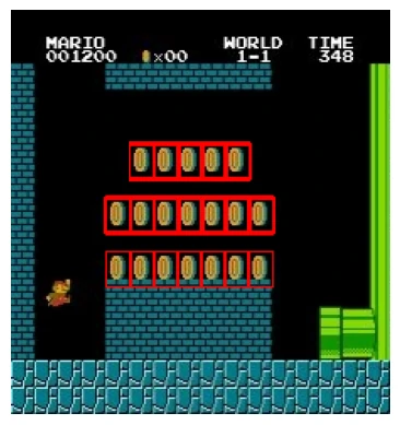
多物体匹配 在这个例子中,将使用著名游戏马里奥的截图,并在其中找到金币
1 2 3 4 5 6 7 8 9 10 11 12 img = cv2.imread("imgs/mario.jpg" ,1 ) img_gray = cv2.cvtColor(img, cv2.COLOR_BGR2GRAY) template = cv2.imread("imgs/mario_coin.jpg" , 0 ) w, h = template.shape[::-1 ] res = cv2.matchTemplate(img_gray, template, cv2.TM_CCOEFF_NORMED) threshold = 0.8 loc= np.where(res>=threshold) for pt in zip (*loc[::-1 ]): cv2.rectangle(img, pt, (pt[0 ]+w,pt[1 ]+h), (0 ,0 ,255 ), 1 ) plt.imshow(cv2.cvtColor(img,cv2.COLOR_BGR2RGB)) plt.axis('off' ) plt.show()
图像拼接 图像拼接的基本流程可以分为以下几个步骤:
图像读取 :读取需要拼接的图像特征点检测 :在每张图像中检测出关键点(特征点)特征点匹配 :在不同图像之间匹配这些特征点计算变换矩阵 :根据匹配的特征点计算图像之间的变换矩阵图像融合 :将图像按照变换矩阵进行拼接,并进行融合处理以消除拼接痕迹
特征点检测是图像拼接的关键步骤,OpenCV 提供了多种特征点检测算法,如SIFT、SURF、ORB 等,其中SIFT和SURF是浮点描述子,ORB是二进制描述子
SIFT长期被认为鲁棒性最好
1 2 3 4 sift = cv2.SIFT_create() kps1, des1 = sift.detectAndCompute(img1, None ) kps2, des2 = sift.detectAndCompute(img2, None )
detectAndCompute() 函数会返回两个值:关键点(keypoints)和描述符(descriptors),关键点是图像中的显著点,描述符是对这些关键点的描述,用于后续的匹配
OpenCV 提供了 BFMatcher 或 FlannBasedMatcher 来进行特征点匹配
匹配方法
描述
SIFT/SURF
ORB/BRIEF
BFMatcher
暴力匹配,逐个对比计算距离
欧式距离(L2范数)
汉明距离(二进制取与)
FlannBasedMatcher
近似快速匹配,使用ANN(近似最相邻)搜索算法
KD-Tree(K维树)
LSH(局部敏感哈希)
BFMatcher简单直接,但计算量大,速度慢;
FlannBasedMatcher匹配速度更快,更适合大规模特征点匹配,虽然结果近似最近邻,但是在实际应用中几乎不影响效果
1 2 3 4 5 6 7 8 bf = cv2.BFMatcher() matches_bf = bf.knnMatch(des1, des2, k=2 ) index_params = dict (algorithm=1 , trees=5 ) search_params = dict (checks=50 ) flann = cv2.FlannBasedMatcher(index_params, search_params) matches_flann = flann.knnMatch(des1, des2, k=2 )
FLANN的创建需要输入参数
SIFT/SURF → algorithm=1, trees=5 (KDTree)
ORB → algorithm=6, table_number=6, key_size=12, multi_probe_level=1 (LSH)
checks=50 → 表示搜索时在多少个叶节点里查找候选(常用 32~128 之间)
knnMatch() 函数会返回每个特征点的两个最佳匹配,通过比率测试(Lowe’s ratio test)来筛选出好的匹配点
1 2 3 4 5 6 good_matches = [] for m, n in matches_flann: if m.distance < 0.75 * n.distance: good_matches.append(m) if len (good_matches) < 10 : raise ValueError("匹配点太少,无法拼接" )
在得到好的匹配点后,可以使用这些点来计算图像之间的变换矩阵
1 2 3 4 5 src_pts = np.float32([kps1[m.queryIdx].pt for m in good_matches]).reshape(-1 , 1 , 2 ) dst_pts = np.float32([kps2[m.trainIdx].pt for m in good_matches]).reshape(-1 , 1 , 2 ) H, mask = cv2.findHomography(src_pts, dst_pts, cv2.RANSAC, 5.0 )
最后使用计算出的单应性矩阵将图像进行拼接,并进行融合处理以消除拼接痕迹
1 2 3 4 5 6 7 8 9 10 11 12 13 14 15 16 17 18 19 h1, w1 = img1.shape[:2 ] h2, w2 = img2.shape[:2 ] pts_img1 = np.float32([[0 ,0 ], [0 ,h1], [w1,h1], [w1,0 ]]).reshape(-1 ,1 ,2 ) pts_img1_trans = cv2.perspectiveTransform(pts_img1, H) pts_all = np.concatenate((pts_img1_trans, np.float32([[0 ,0 ],[0 ,h2],[w2,h2],[w2,0 ]]).reshape(-1 ,1 ,2 )), axis=0 ) [xmin, ymin] = np.int32(pts_all.min (axis=0 ).ravel() - 0.5 ) [xmax, ymax] = np.int32(pts_all.max (axis=0 ).ravel() + 0.5 ) t = [-xmin, -ymin] H_trans = np.array([[1 ,0 ,t[0 ]], [0 ,1 ,t[1 ]], [0 ,0 ,1 ]]) result = cv2.warpPerspective(img1, H_trans.dot(H), (xmax-xmin, ymax-ymin)) result[t[1 ]:h2+t[1 ], t[0 ]:w2+t[0 ]] = img2
拼接效果可能不是特别好
简单滤镜 主要滤镜效果:
滤镜效果 实现方法
灰度滤镜
cv2.cvtColor(image, cv2.COLOR_BGR2GRAY)
模糊滤镜
cv2.GaussianBlur(image, (15, 15), 0)
怀旧滤镜
通过调整色彩通道的权重,模拟老照片效果
浮雕滤镜
使用卷积核 [[-2, -1, 0], [-1, 1, 1], [0, 1, 2]] 进行卷积操作
锐化滤镜
使用卷积核 [[0, -1, 0], [-1, 5, -1], [0, -1, 0]] 进行卷积操作
边缘检测滤镜
cv2.Canny(gray_image, 100, 200)
怀旧滤镜 1 2 3 4 5 6 7 8 9 10 img = cv2.imread("imgs/LenaRGB.bmp" ) b,g,r = cv2.split(img) r = np.clip(r*0.393 +g*0.769 +b*0.189 ,0 ,255 ).astype(np.uint8) g = np.clip(r*0.349 +g*0.686 +b*0.168 ,0 ,255 ).astype(np.uint8) b = np.clip(r*0.272 +g*0.534 +b*0.131 ,0 ,255 ).astype(np.uint8) img = cv2.merge([b,g,r]) plt.imshow(cv2.cvtColor(img, cv2.COLOR_BGR2RGB))
浮雕滤镜 浮雕滤镜通过计算图像中相邻像素的差值,生成一种类似于浮雕的效果,这种滤镜通常用于增强图像的边缘和纹理
1 2 3 4 5 6 7 8 9 10 11 img = cv2.imread("imgs/LenaRGB.bmp" ) gray = cv2.cvtColor(img, cv2.COLOR_BGR2GRAY) kernel = np.array([[-2 , -1 , 0 ], [-1 , 1 , 1 ], [0 , 1 , 2 ]]) emboss_img = cv2.filter2D(gray, -1 , kernel) plt.imshow(cv2.cvtColor(emboss_img, cv2.COLOR_BGR2RGB)) plt.axis("off" )
霍夫变换 霍夫变换常用来在图像中提取直线和圆等几何形状
霍夫直线变换 直线的参数方程:$y=kx+b$
但是在 $k\rightarrow \infty$ 时将无效,霍夫变换用极坐标的形式
用cv2.HoughLines()在二值图上实现霍夫变换,函数返回的是一组直线的$(\rho ,\theta)$数据
1 lines = cv2.HoughLines(edges, 1 , np.pi / 180 , threshold)
参数1:一般是边缘检测后的二值图
参数2:距离$\rho$的精度,值越大,考虑越多的线,一般使用1像素
参数3:角度$\theta $的精度,值越小,考虑越多的线,一般使用1度
参数4:累加数阈值,值越小,考虑越多的线
标准霍夫变换 会检测到整条无穷延伸的直线,而实际中更想要线段
OpenCV 提供 cv2.HoughLinesP(统计概率霍夫直线变换),这是一种改进算法,输出线段的起止点
1 linesP = cv2.HoughLinesP(edges, 1 , np.pi/180 , threshold, minLineLength=50 , maxLineGap=10 )
前面几个参数跟之前的一样,有两个可选参数,最短长度阈值以及同一直线两点间的最大距离
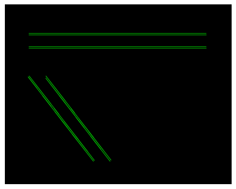
读取 → 转灰度 → Canny检测 → 霍夫变换
1 2 3 4 5 6 7 8 9 10 11 12 13 import cv2import matplotlib.pyplot as pltimport numpy as npimg = cv2.imread("imgs/hough_test.jpg" ) drawing = np.zeros(img.shape[:], dtype=np.uint8) gray = cv2.cvtColor(img, cv2.COLOR_BGR2GRAY) edges = cv2.Canny(gray, 50 , 150 ) linesP = cv2.HoughLinesP(edges, 1 , np.pi/180 , 80 , minLineLength=50 , maxLineGap=10 ) for x1, y1, x2, y2 in linesP[:,0 ]: cv2.line(drawing, (x1,y1), (x2,y2), (0 ,255 ,0 ), 2 ) plt.imshow(drawing)
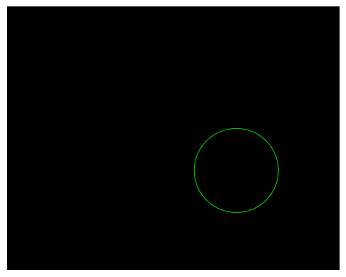
霍夫圆变换 同理,霍夫变换也可以用于检测圆
1 2 3 4 5 6 7 8 9 10 cv2.HoughCircles( image, method, dp, minDist, param1=100 , param2=30 , minRadius=0 , maxRadius=0 )
1 2 3 4 5 6 7 8 9 10 11 img = cv2.imread("imgs/hough_test.jpg" ) drawing = np.zeros(img.shape[:], dtype=np.uint8) gray = cv2.cvtColor(img, cv2.COLOR_BGR2GRAY) h,w = gray.shape circles = cv2.HoughCircles(gray, cv2.HOUGH_GRADIENT, dp = 1 , minDist= h/8 , param2=30 ) circles = np.uint16(np.around(circles)) for (x, y, r) in circles[0 , :]: cv2.circle(drawing, (x, y), r, (0 , 255 , 0 ), 2 ) plt.imshow(drawing) plt.axis("off" )
视频处理 视频是由一系列连续的图像帧组成的,每一帧都是一幅静态图像,核心就是对这些图像帧进行处理
视频读取 要读取视频文件,首先需要创建一个 cv2.VideoCapture 对象,并指定视频文件的路径
1 2 3 4 5 6 7 8 9 10 11 12 13 14 15 16 cap = cv2.VideoCapture("imgs/camera_vedio.mp4" ) if not cap.isOpened(): print ("Error: Could not open video." ) exit() while True : ret, frame = cap.read() if not ret: break cv2.imshow('Video' , frame) if cv2.waitKey(25 ) & 0xFF == ord ('q' ): break cap.release() cv2.destroyAllWindows()
除了读取视频文件,OpenCV 还可以直接从摄像头读取视频,只需要将 cv2.VideoCapture 的参数设置为摄像头的索引(通常为0)即可:
1 2 3 4 5 6 7 8 9 10 11 12 13 14 15 16 17 18 cap = cv2.VideoCapture(0 ) if not cap.isOpened(): print ("Error: Could not open camera." ) exit() while True : ret, frame = cap.read() if not ret: break cv2.imshow('Camera' , frame) if cv2.waitKey(25 ) & 0xFF == 27 : break cap.release() cv2.destroyAllWindows()
电脑没有摄像头的话可以参考这篇内容:虚拟摄像头构建
之后就可以对视频画面进行一些实时操作了
视频帧处理 在读取视频帧后,可以对每一帧进行各种图像处理操作,并进行保存
在读取后需要利用.get()获取视频的属性(如宽度、高度、帧率等),方便创建保存对象
1 2 3 fps = int (cap.get(cv2.CAP_PROP_FPS)) width = int (cap.get(cv2.CAP_PROP_FRAME_WIDTH)) height = int (cap.get(cv2.CAP_PROP_FRAME_HEIGHT))
视频如果分辨率和帧率过高输出可能会出现掉帧,根据性能量力而行
1 2 3 4 5 6 7 8 9 10 11 12 13 14 15 16 17 18 19 20 21 22 23 24 25 26 27 28 29 30 31 32 33 34 import cv2input_path = "imgs/tree.mp4" output_path = "tree.avi" cap = cv2.VideoCapture(input_path) if not cap.isOpened(): print ("Error: Could not open camera." ) exit() fps = int (cap.get(cv2.CAP_PROP_FPS)) fourcc = cv2.VideoWriter_fourcc(*'XVID' ) out = cv2.VideoWriter(output_path, fourcc, fps, (1080 , 720 )) while True : ret, frame = cap.read() if not ret: break frame = cv2.resize(frame, (1080 ,720 )) gray = cv2.cvtColor(frame, cv2.COLOR_BGR2GRAY) blur = cv2.GaussianBlur(gray, (5 ,5 ), 0 ) edges = cv2.Canny(blur, 50 , 150 ) edges = cv2.cvtColor(edges, cv2.COLOR_GRAY2BGR) out.write(edges) cap.release() out.release() cv2.destroyAllWindows() print ("视频处理完毕" )
摄像头实时处理读出:
1 2 3 4 5 6 7 8 9 10 11 12 13 14 15 16 17 18 19 20 21 22 23 24 25 26 27 28 29 30 31 import cv2output_path = "res/camera_output.mp4" cap = cv2.VideoCapture(0 ) if not cap.isOpened(): print ("Error: Could not open camera." ) exit() fps = 30.0 width = int (cap.get(cv2.CAP_PROP_FRAME_WIDTH)) height = int (cap.get(cv2.CAP_PROP_FRAME_HEIGHT)) fourcc = cv2.VideoWriter_fourcc(*'mp4v' ) out = cv2.VideoWriter(output_path, fourcc, fps, (width, height)) print ("按 ESC 退出录制..." )while True : ret, frame = cap.read() if not ret: break gray = cv2.cvtColor(frame, cv2.COLOR_BGR2GRAY) edges = cv2.Canny(gray, 50 , 150 ) edges = cv2.cvtColor(edges, cv2.COLOR_GRAY2BGR) out.write(edges) cv2.imshow("Camera Processed" , edges) if cv2.waitKey(1 ) & 0xFF == 27 : break cap.release() out.release() cv2.destroyAllWindows() print ("录制结束,视频保存为:" , output_path)
物体检测 OpenCV提供了多种物体检测算法,如 Haar 特征分类器、HOG + SVM 等
Haar特征分类器 Haar 特征分类器是一种基于 Haar-like 特征的机器学习方法,用于检测图像中的目标
OpenCV 提供了预训练的 Haar 特征分类器,cv2.CascadeClassifier用于加载分类器,参数是分类器文件的路径
模型文件
检测目标
描述
haarcascade_frontalface_default.xml正面人脸
最常用
haarcascade_profileface.xml侧面人脸
haarcascade_eye.xml眼睛检测
需要配合人脸使用
haarcascade_smile.xml微笑检测
进行人脸检测:
1 2 3 4 5 6 7 8 9 10 11 12 13 14 15 16 17 18 19 20 21 22 23 24 25 import cv2face_cascade = cv2.CascadeClassifier(cv2.data.haarcascades + 'haarcascade_frontalface_default.xml' ) cap = cv2.VideoCapture(0 ) while True : ret, frame = cap.read() if not ret: break gray_frame = cv2.cvtColor(frame, cv2.COLOR_BGR2GRAY) faces = face_cascade.detectMultiScale( gray_frame, scaleFactor=1.1 , minNeighbors=5 , minSize=(30 , 30 )) for (x, y, w, h) in faces: cv2.rectangle(frame, (x, y), (x+w, y+h), (255 , 0 , 0 ), 2 ) cv2.imshow('Face Detection' , frame) if cv2.waitKey(25 ) & 0xFF == 27 : break cap.release() cv2.destroyAllWindows()
detectMultiScale会返回所有检测到的矩形框 (x, y, w, h)
scaleFactor:表示图像尺寸的缩小比例,>1缩小图像,常用1.1
计算方法:缩小比例 = 1 - (1/scaleFactor)
scaleFactor=1.1 时,每次缩放后的新尺寸 = 原尺寸×(1/1.1) ≈ 原尺寸×0.909
minNeighbors:表示在当前强度中心周围有多少个目标同时检测到才算有效,值越高越严格
minSize:最小检测窗口,表示目标的最小尺寸
Haar属于传统CV算法,速度快,适合实时,但检测精度不如深度学习模型,对光照、角度变化不鲁棒
YOLOv5 相比Haar,Yolov5可同时检测80+类别物体,输出带类别标签的边界框,对部分遮挡、光照变化、背景杂乱有较强鲁棒性,训练后的代码简洁
1 2 3 4 5 6 7 8 9 10 11 12 13 14 15 16 17 18 19 20 import cv2import torchimport warningswarnings.filterwarnings("ignore" , category=FutureWarning, message=".*torch.cuda.amp.autocast.*" ) model = torch.hub.load('ultralytics/yolov5' , 'yolov5s' ) cap = cv2.VideoCapture(0 ) while True : ret, frame = cap.read() if not ret: break results = model(frame) annotated_frame = results.render()[0 ] cv2.imshow("YOLOv5 Real Time Detection" , annotated_frame) if cv2.waitKey(30 ) & 0xFF == 27 : break cap.release() cv2.destroyAllWindows()
运动检测 帧差法 通过计算帧之间的差异来检测运动物体,最直观
特点:简单,适合物体比较大、背景稳定的场景
1 2 3 4 5 6 7 8 9 10 11 12 13 14 15 16 17 18 19 20 21 22 23 24 25 26 27 28 29 30 31 32 33 34 35 import cv2cap = cv2.VideoCapture(0 ) ret, prev_frame = cap.read() prev_gray = cv2.cvtColor(prev_frame, cv2.COLOR_BGR2GRAY) prev_gray = cv2.GaussianBlur(prev_gray, (5 , 5 ), 0 ) while cap.isOpened(): ret, frame = cap.read() if not ret: break gray = cv2.cvtColor(frame, cv2.COLOR_BGR2GRAY) gray = cv2.GaussianBlur(gray, (5 , 5 ), 0 ) diff = cv2.absdiff(prev_gray, gray) _, thresh = cv2.threshold(diff, 25 , 255 , cv2.THRESH_BINARY) dilated = cv2.dilate(thresh, None , iterations=2 ) contours, _ = cv2.findContours(dilated, cv2.RETR_EXTERNAL, cv2.CHAIN_APPROX_SIMPLE) for cnt in contours: if cv2.contourArea(cnt) < 500 : continue x, y, w, h = cv2.boundingRect(cnt) cv2.rectangle(frame, (x, y), (x+w, y+h), (0 , 255 , 0 ), 2 ) cv2.imshow("motion detection" , frame) prev_gray = gray if cv2.waitKey(1 ) & 0xFF == 27 : break cap.release() cv2.destroyAllWindows()
背景减除法 背景减除法是一种更为精准和鲁棒的运动检测技术,通过学习视频的静态背景,然后将当前帧与背景模型进行比较,从而识别出前景(即运动的物体),它比帧差法稳定,对光照变化更鲁棒
其基本流程如下:
背景建模:通过分析视频序列中的多帧图像,建立一个背景模型
前景检测:将当前帧与背景模型进行比较,找出与背景差异较大的区域,这些区域即为前景对象。
背景更新:随着时间的推移,背景可能会发生变化(如光照变化、背景物体的移动等),因此需要不断更新背景模型
OpenCV 提供了多种背景减除算法,其中MOG和MOG2是最常用的两种方法
MOG2是MOG的改进版本,主要区别在于它能够自动选择高斯分布的数量,并且能够更好地适应背景的变化
1 fgbg = cv2.createBackgroundSubtractorMOG2(history=500 , varThreshold=16 , detectShadows=True )
history:训练的帧数(默认500),值大表示模型记忆更久,适合稳定场景;值小更灵敏,适合背景经常变化的环境
varThreshold:像素和背景模型的阈值(默认 16)
值小 → 更容易检测出前景,但噪声也多;值大 → 只检测明显运动的物体
detectShadows:是否检测阴影,默认True,如果只想要前景物体,可以关掉它
1 fgmask = fgbg.apply(frame)
输入一帧图像,输出前景掩码(mask),掩码是单通道图像:背景0,前景255,阴影127
1 2 3 4 5 6 7 8 9 10 11 12 13 14 15 16 17 18 19 20 21 22 23 24 25 26 27 28 29 30 31 32 33 34 35 36 import cv2import numpy as npcap = cv2.VideoCapture(0 ) fgbg = cv2.createBackgroundSubtractorMOG2(history=500 , varThreshold=50 , detectShadows=False ) while True : ret, frame = cap.read() if not ret: break fgmask = fgbg.apply(frame) kernel = cv2.getStructuringElement(cv2.MORPH_ELLIPSE, (3 , 3 )) fgmask = cv2.morphologyEx(fgmask, cv2.MORPH_OPEN, kernel) kernel = cv2.getStructuringElement(cv2.MORPH_ELLIPSE, (7 , 7 )) fgmask = cv2.dilate(fgmask, kernel) contours, hierarchy = cv2.findContours(fgmask, cv2.RETR_EXTERNAL, cv2.CHAIN_APPROX_SIMPLE) for contour in contours: if cv2.contourArea(contour) < 500 : continue (x, y, w, h) = cv2.boundingRect(contour) cv2.rectangle(frame, (x, y), (x+w, y+h), (0 , 255 , 0 ), 2 ) cv2.imshow('Original Frame' , frame) cv2.imshow('Foreground Mask' , fgmask) if cv2.waitKey(1 ) & 0xff == 27 : break cap.release() cv2.destroyAllWindows()
卷积核大小不同是为了先用最小的代价去除噪声,再用足够的强度来恢复和增强目标
会发现在检测时一个人可能出现多个框,是因为这个算法并不会把人当作一个整体来看待
相比YOLO这只是一种比较简单的低级检测,只会发现哪里在动,不关心这是不是一个整体
车道检测 无人车上的相机拍摄的视频中,车道线的位置应该基本固定在某一个范围内
手动把这部分 ROI 区域抠出来,就会排除掉大部分干扰
利用霍夫变换检测直线,但 ROI 区域内的边缘直线信息还是很多。考虑到只有左右两条车道线,一条斜率为正,一条为负,可将所有的线分为两组,每组再通过均值或最小二乘法拟合的方式确定唯一一条线就可以完成检测
总体步骤如下:
读取视频帧(逐帧处理)
灰度化 + 高斯滤波(降噪)
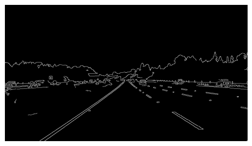
Canny边缘检测(提取边缘)
定义ROI(只保留车道区域)
霍夫直线变换(检测车道线)
线段拟合与绘制(平滑显示结果)
图像预处理 1 2 3 4 5 6 7 8 9 10 11 blur_ksize = 5 canny_low = 50 canny_high = 150 def process_img (img ): gray = cv2.cvtColor(img, cv2.COLOR_BGR2GRAY) blur = cv2.GaussianBlur(gray, (blur_ksize,blur_ksize), 0 ) edges = cv2.Canny(blur, canny_low, canny_high) return edges
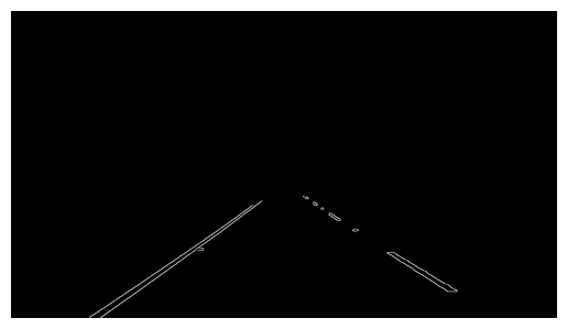
ROI截取 创建一个梯形的 mask 掩膜,然后与边缘检测结果图混合运算
掩膜中白色的部分保留,黑色的部分舍弃
1 2 3 4 5 6 7 8 9 10 11 def roi_mask (img, vertices ): mask = np.zeros_like(img) cv2.fillPoly(mask, vertices, 255 ) masked_image = cv2.bitwise_and(img, mask) return masked_image h, w = edges.shape[:2 ] roi_vertices = np.array([[(0 ,h),(460 , 325 ), (520 , 325 ),(w,h)]]) roi = roi_mask(edges, roi_vertices)
霍夫直线提取 使用统计概率霍夫直线变换,因为后续还需要处理
1 2 3 4 5 6 7 8 9 10 11 12 13 14 def draw_lines (img, lines, color=[255 , 0 , 0 ], thickness=1 ): if lines is None : return for x1, y1, x2, y2 in lines[:,0 ]: cv2.line(img, (x1, y1), (x2, y2), color, thickness) rho = 1 theta = np.pi / 180 threshold = 15 min_line_len = 40 max_line_gap = 20 lines = cv2.HoughLinesP(roi, rho, theta, threshold, minLineLength=min_line_len, maxLineGap=max_line_gap) drawing = np.zeros(img.shape[:], dtype=np.uint8) draw_lines(drawing, lines)
车道计算 前面通过霍夫变换得到了多条直线的起点和终点
目的是通过某种算法只得到左右两条车道线
根据斜率正负划分某条线是左车道还是右车道
迭代计算各直线斜率与斜率均值的差,排除掉差值过大的异常数据
最小二乘法拟合左右车道线
Python 中可以直接使用np.polyfit()进行最小二乘法拟合
1 2 3 4 5 6 7 8 9 10 11 12 13 14 15 16 17 18 19 20 21 22 23 24 25 26 27 28 29 30 31 32 33 34 35 36 37 38 39 40 41 42 43 44 45 46 47 48 49 50 51 52 53 54 55 56 57 58 59 60 61 62 63 64 65 66 67 68 69 70 71 72 73 74 75 76 77 def clean_lines (lines, threshold ): slopes = [] for line in lines: arr = np.array(line).reshape(4 ) x1, y1, x2, y2 = arr if x2 == x1: continue slope = (y2 - y1) / (x2 - x1) slopes.append(slope) slopes = np.array(slopes) mean_slope = np.mean(slopes) mask = np.abs (slopes - mean_slope) < threshold return [line for line, sign in zip (lines, mask) if sign] def least_squares_fit (point_list, ymin, ymax ): if not point_list or len (point_list) < 2 : return None x = [p[0 ] for p in point_list] y = [p[1 ] for p in point_list] fit = np.polyfit(y, x, 1 ) fit_fn = np.poly1d(fit) xmin = int (fit_fn(ymin)) xmax = int (fit_fn(ymax)) return [(xmin, ymin), (xmax, ymax)] def draw_lanes (img, lines, color=[0 , 255 , 0 ], thickness=8 ): h = img.shape[0 ] left_lines, right_lines = [], [] for line in lines: for x1, y1, x2, y2 in line: if x2 == x1: continue k = (y2 - y1) / (x2 - x1) if k < 0 : left_lines.append(line) else : right_lines.append(line) if not left_lines or not right_lines: return left_lines = clean_lines(left_lines, 0.1 ) right_lines = clean_lines(right_lines, 0.1 ) left_points = [] for l in left_lines: x1, y1, x2, y2 = l.reshape(4 ) left_points.append((x1, y1)) left_points.append((x2, y2)) right_points = [] for l in right_lines: x1, y1, x2, y2 = l.reshape(4 ) right_points.append((x1, y1)) right_points.append((x2, y2)) left_results = least_squares_fit(left_points, 325 , h) right_results = least_squares_fit(right_points, 325 , h) if left_results is None or right_results is None : return vtxs = np.array([[left_results[0 ], left_results[1 ], right_results[1 ], right_results[0 ]]]) cv2.fillPoly(img, vtxs, color)
视频处理 搞定图以后就是视频帧的提取和合成
1 2 3 4 5 6 7 8 9 10 11 12 13 14 15 16 17 18 19 20 21 22 23 cap = cv2.VideoCapture("Lane_Detection/cv2_yellow_lane.mp4" ) fourcc = cv2.VideoWriter_fourcc(*'mp4v' ) fps = cap.get(cv2.CAP_PROP_FPS) w = int (cap.get(cv2.CAP_PROP_FRAME_WIDTH)) h = int (cap.get(cv2.CAP_PROP_FRAME_HEIGHT)) out = cv2.VideoWriter("Lane_Detection/output.mp4" , fourcc, fps, (w, h)) while cap.isOpened(): ret, frame = cap.read() if not ret: break result = process_img(frame) cv2.imshow("Lane Detection" , result) out.write(result) if cv2.waitKey(30 ) & 0xFF == 27 : break cap.release() out.release() cv2.destroyAllWindows()
也可以利用Python 的视频编辑包moviepy
1 2 3 4 output = 'Lane_Detection/output.mp4' clip = VideoFileClip("Lane_Detection/cv2_yellow_lane.mp4" ) out_clip = clip.fl_image(process_img) out_clip.write_videofile(output, audio=False )
全代码 1 2 3 4 5 6 7 8 9 10 11 12 13 14 15 16 17 18 19 20 21 22 23 24 25 26 27 28 29 30 31 32 33 34 35 36 37 38 39 40 41 42 43 44 45 46 47 48 49 50 51 52 53 54 55 56 57 58 59 60 61 62 63 64 65 66 67 68 69 70 71 72 73 74 75 76 77 78 79 80 81 82 83 84 85 86 87 88 89 90 91 92 93 94 95 96 97 98 99 100 101 102 103 104 105 106 107 108 109 110 111 112 113 114 115 116 117 118 119 120 121 122 123 124 125 126 127 128 129 130 131 132 133 134 135 136 137 138 139 140 141 142 143 144 145 146 147 148 149 150 151 152 153 154 155 156 157 158 159 160 161 162 import cv2import numpy as npfrom moviepy.editor import VideoFileClipblur_ksize = 5 canny_low = 50 canny_high = 150 rho = 1 theta = np.pi / 180 threshold = 15 min_line_len = 40 max_line_gap = 20 def roi_mask (img, vertices ): mask = np.zeros_like(img) cv2.fillPoly(mask, vertices, 255 ) masked_image = cv2.bitwise_and(img, mask) return masked_image def draw_lines (img, lines, color=[255 , 0 , 0 ], thickness=1 ): if lines is None : return for x1, y1, x2, y2 in lines[:,0 ]: cv2.line(img, (x1, y1), (x2, y2), color, thickness) def clean_lines (lines, threshold ): slopes = [] for line in lines: arr = np.array(line).reshape(4 ) x1, y1, x2, y2 = arr if x2 == x1: continue slope = (y2 - y1) / (x2 - x1) slopes.append(slope) slopes = np.array(slopes) mean_slope = np.mean(slopes) mask = np.abs (slopes - mean_slope) < threshold return [line for line, sign in zip (lines, mask) if sign] def least_squares_fit (point_list, ymin, ymax ): if not point_list or len (point_list) < 2 : return None x = [p[0 ] for p in point_list] y = [p[1 ] for p in point_list] fit = np.polyfit(y, x, 1 ) fit_fn = np.poly1d(fit) xmin = int (fit_fn(ymin)) xmax = int (fit_fn(ymax)) return [(xmin, ymin), (xmax, ymax)] def draw_lanes (img, lines, color=[0 , 255 , 0 ], thickness=8 ): h = img.shape[0 ] left_lines, right_lines = [], [] for line in lines: for x1, y1, x2, y2 in line: if x2 == x1: continue k = (y2 - y1) / (x2 - x1) if k < 0 : left_lines.append(line) else : right_lines.append(line) if not left_lines or not right_lines: return left_lines = clean_lines(left_lines, 0.1 ) right_lines = clean_lines(right_lines, 0.1 ) left_points = [] for l in left_lines: x1, y1, x2, y2 = l.reshape(4 ) left_points.append((x1, y1)) left_points.append((x2, y2)) right_points = [] for l in right_lines: x1, y1, x2, y2 = l.reshape(4 ) right_points.append((x1, y1)) right_points.append((x2, y2)) left_results = least_squares_fit(left_points, 325 , h) right_results = least_squares_fit(right_points, 325 , h) if left_results is None or right_results is None : return vtxs = np.array([[left_results[0 ], left_results[1 ], right_results[1 ], right_results[0 ]]]) cv2.fillPoly(img, vtxs, color) def process_img (img ): h, w = img.shape[:2 ] gray = cv2.cvtColor(img, cv2.COLOR_BGR2GRAY) blur = cv2.GaussianBlur(gray, (blur_ksize,blur_ksize), 0 ) edges = cv2.Canny(blur, canny_low, canny_high) roi_vertices = np.array([[(0 ,h),(460 , 325 ), (520 , 325 ),(w,h)]]) roi = roi_mask(edges, roi_vertices) lines = cv2.HoughLinesP(roi, rho, theta, threshold, minLineLength=min_line_len, maxLineGap=max_line_gap) drawing = np.zeros_like(img) draw_lanes(drawing, lines) result = cv2.addWeighted(img, 0.9 , drawing, 0.4 , 0 ) return result if __name__ == "__main__" : cap = cv2.VideoCapture("Lane_Detection/cv2_yellow_lane.mp4" ) fourcc = cv2.VideoWriter_fourcc(*'mp4v' ) fps = cap.get(cv2.CAP_PROP_FPS) w = int (cap.get(cv2.CAP_PROP_FRAME_WIDTH)) h = int (cap.get(cv2.CAP_PROP_FRAME_HEIGHT)) out = cv2.VideoWriter("Lane_Detection/output.mp4" , fourcc, fps, (w, h)) while cap.isOpened(): ret, frame = cap.read() if not ret: break result = process_img(frame) cv2.imshow("Lane Detection" , result) out.write(result) if cv2.waitKey(30 ) & 0xFF == 27 : break cap.release() out.release() cv2.destroyAllWindows() """ output = 'Lane_Detection/output.mp4' clip = VideoFileClip("Lane_Detection/cv2_yellow_lane.mp4") out_clip = clip.fl_image(process_img) out_clip.write_videofile(output, audio=False) """

 (1).png)

.webp)